Self-Supervised Learning(SSL)

Introduction to Self-Supervised Learning (SSL)

Technical terms

Supervised Learning: using data with fine-grained human-annotated labels to train AI models.
Semi-supervised Learning: using a small amount of labeled data and a large amount of unlabeled data.

Weakly-supervised Learning: using data with coarse-grained labels or inaccurate labels.
The cost of making weak supervision labels is generally much cheaper than fine-grained labels for supervised methods.
e.g. label tiger, cat, dog as ‘animal’
Unsupervised Learning: learning methods without using any human-annotated labels.

• Self-supervised Learning: models are explicitly trained with automatically generated labels.
  The learned features can be transferred to multiple different tasks.
  Self-supervised learning is a subset of unsupervised learning.

Motivation of self-supervised learning

Hard/expensive to obtain annotation.
Untapped/availability of vast numbers of unlabelled data.
Instead of relying on annotations, self-supervised learning generates labels from data by discovering relationships between the data - a step believed to be critical to achieve human-level intelligence.

Learning visual representations without human supervision

• Generative approaches
  It learns to generate or otherwise model pixels in the input space.
  Pixel-level generation is computationally expensive and may not be necessary for representation learning.
• Discriminative approaches
  It learns representations using objective functions similar to those used for supervised learning.
  It trains networks to perform pretext tasks where both the inputs and labels are derived from an unlabeled dataset.
  Many such approaches used heuristics to design pretext tasks, which could limit the generality of the learned representations.
  Discriminative approaches based on contrastive learning in the latent space have recently shown great promise, achieving great results.

Define a Pretext Task or Proxy Task

• Pretext Task (Proxy task)
  Pre-designed tasks for networks to solve, and features are learned by learning objective functions of pretext tasks.
• Downstream Task
  Applications that are used to evaluate the quality of features learned by self-supervised learning.
  These applications can greatly benefit from the pretrained models when training data are not enough.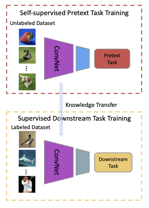
  

Examples of Pretext Task

• Colourization
  CNN model learns to predict colours from a greyscale image.
• Placing image patches in the right place
  The patches are extracted from an image and shuffled.
  The model learns to solve this jigsaw and arrange the patches in the correct sequence.
• Placing frames in the right order
  The model learns to sort the shuffled frames in a video sequence.

SimCLR: state-of-the-art SSL framework

The Intuition behind Contrastive Learning

No need to know the exact label of an image.
Only need to tell which images are similar and which are different:

• Examples of similar and dissimilar images
• Ability to know what an image represents
• Ability to quantify if two images are similar

Similar and dissimilar images

We need example pairs of images that are similar and images that are different to train a model.
We need some techniques to get representations that allow the machine to understand an image - to find the pattern.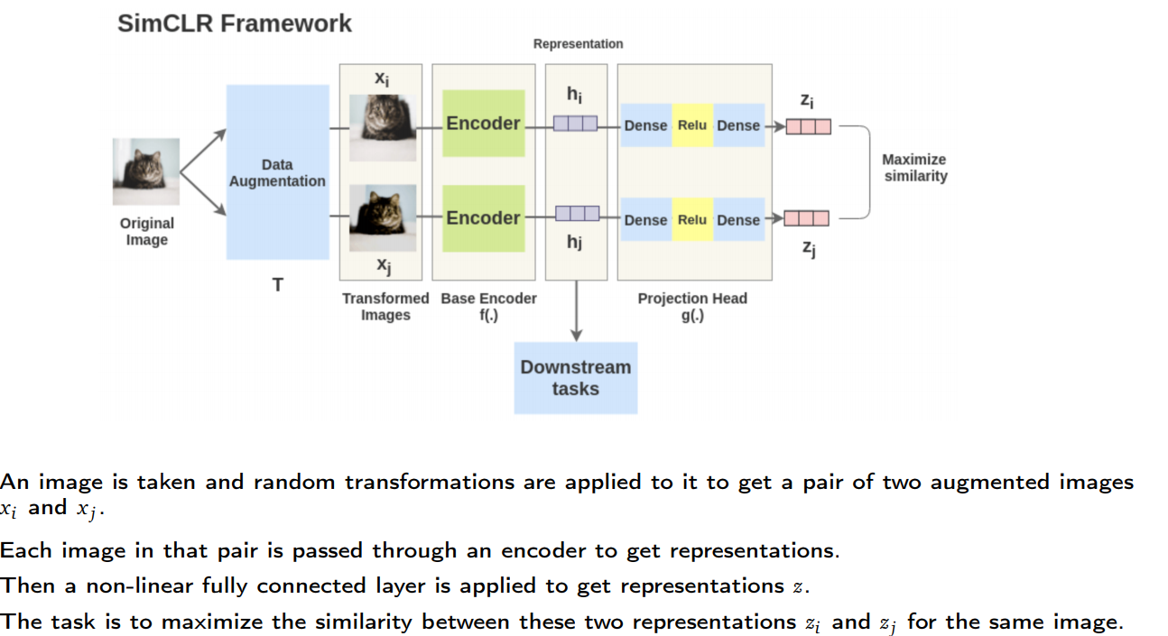

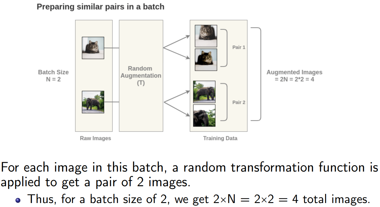
Step-by-step example of SimCLR

Self-supervised Formulation [Data Augmentation]

Getting Representations [Base Encoder]

Each augmented image in a pair is passed through an encoder to get image representations.
The encoder is general and replaceable with other architectures.
The two encoders have shared weights and we get vectors $h_i$ and $h_j$.
For example, the authors used ResNet-50 architecture as the ConvNet encoder and the output is a 2048-dimensional vector h.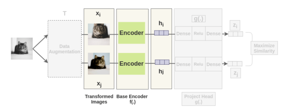

Projection Head

The representations $h_i$ and $h_j$ of the two augmented images are then passed through several non-linear Dense → Relu → Dense
layers to apply non-linear transformation and project it into a representation $z_i$ and $z_j$(embedding vector for augmebted images).
This is denoted by $g(.)$ in the paper and called projection head.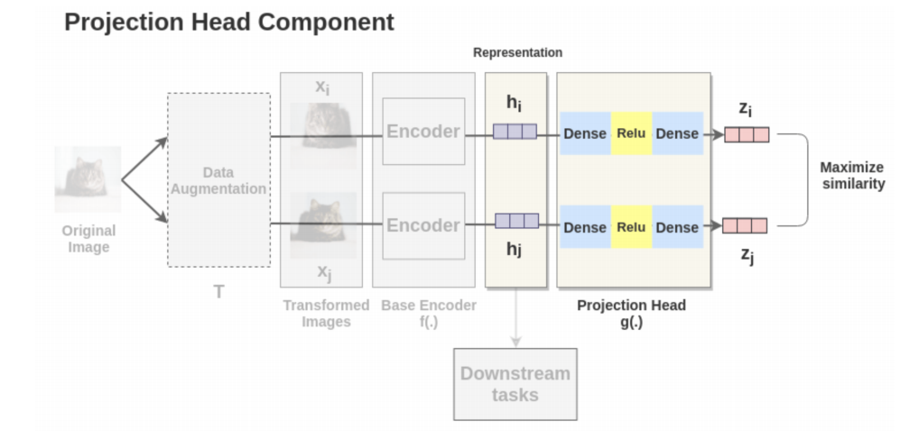

Tuning Model: [Bringing similar closer]

Calculation of Cosine Similarity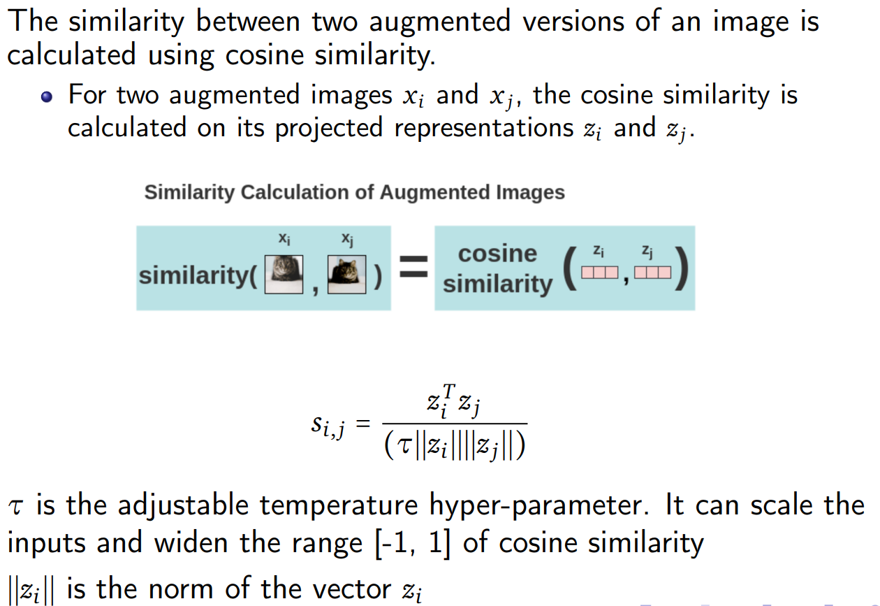

Loss Calculation
SimCLR uses a contrastive loss called “NT-Xent loss” (Normalized Temperature-Scaled Cross-Entropy Loss).

• First, the augmented pairs in the batch are taken one by one.
• Next, we apply the softmax function to get the probability of these two images being similar.
  This softmax calculation is equivalent to getting the probability of the second augmented cat image being the most similar to the first
  cat image in the pair.
  Here, all remaining images in the batch are sampled as a dissimilar image (negative pair).
  Thus, we don’t need specialized architecture, memory bank or queue need by previous approaches like InstDisc, MoCo or PIRL.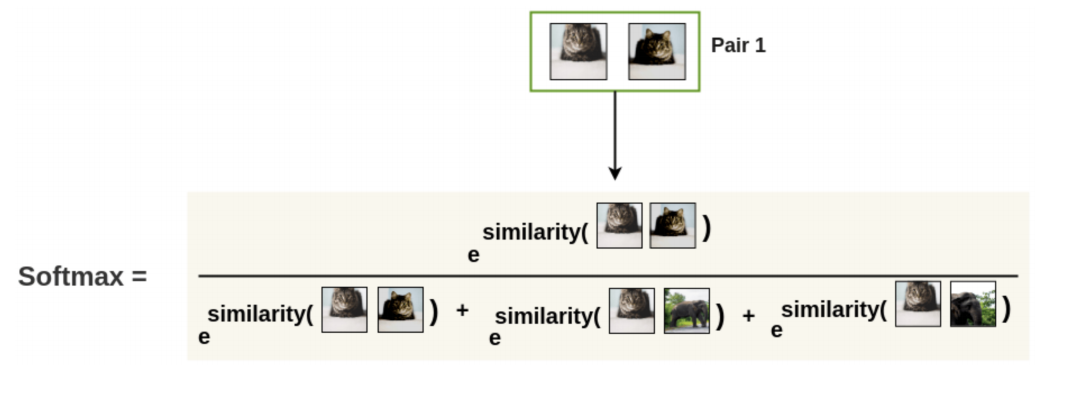
  
• Then, the loss is calculated for a pair by taking the negative of the log of the Softmax calculation.
  This formulation is the Noise Contrastive Estimation(NCE) Loss.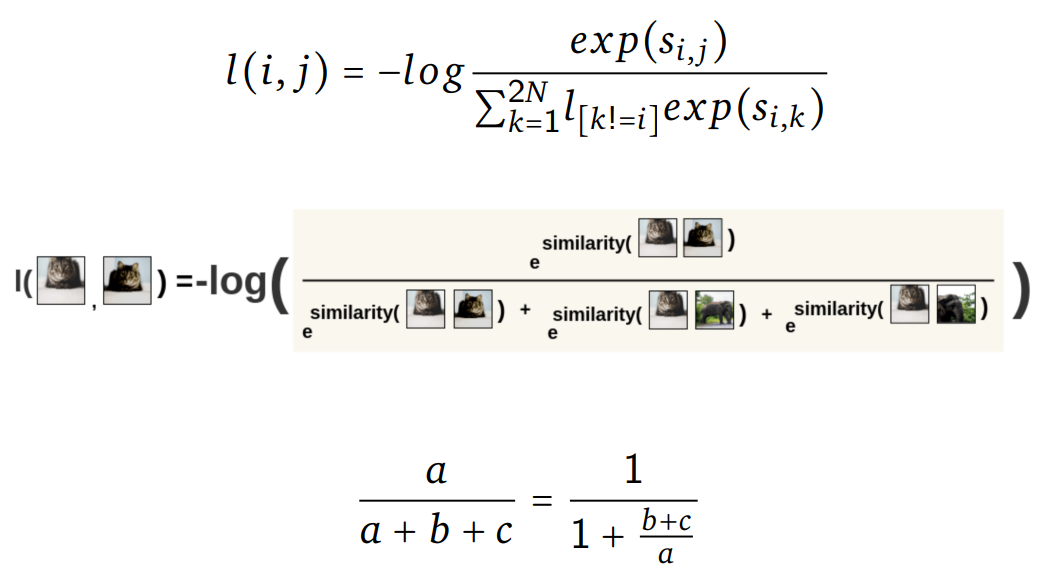
  
  We interchange the positions of the images and calculate the loss for the same pair again.
• Finally, we compute loss over all the pairs in the batch of size $N$ and take an average.
  Based on the loss, the encoder and projection head representations improves over time.
  The representations obtained place similar images closer.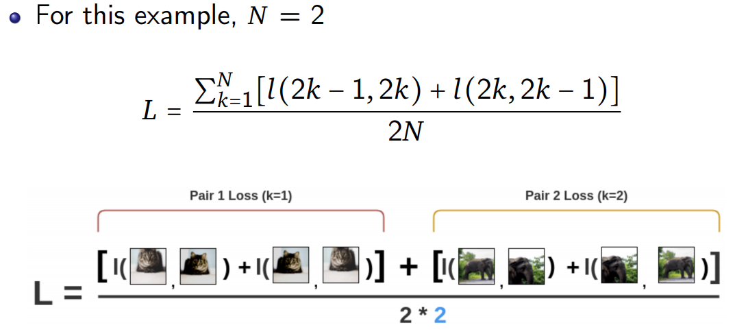
  

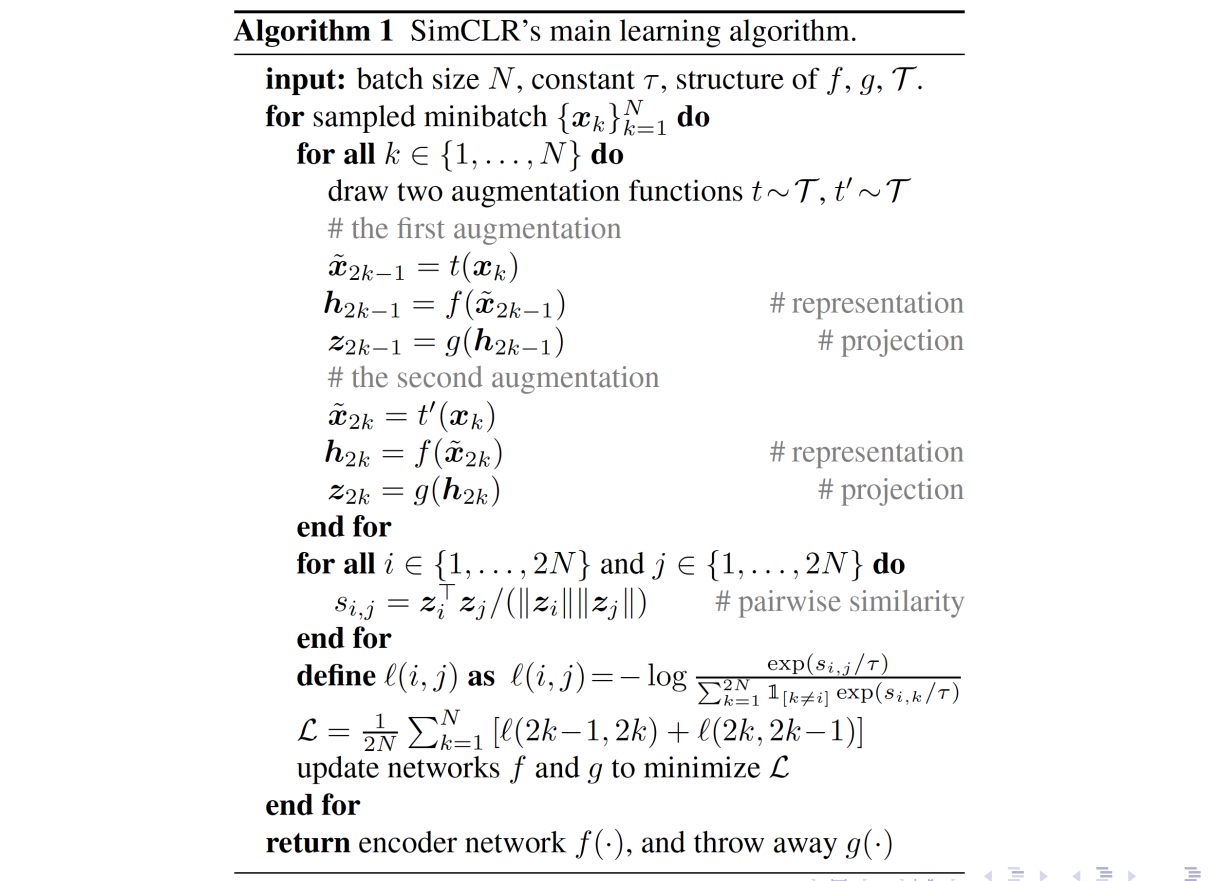
SimCLR Algorithm

4 major components of SimCLR

A stochastic data augmentation module that transforms any given data example randomly resulting in two correlated views of the same example, denoted $\tilde{x}_i$ and $\tilde{x}_j$ (positive pair).

• SimCLR sequentially applied 3 simple augmentations:
  random cropping followed by resize back to the original size
  random color distortions
  random Gaussian blur
• The combination of random crop and color distortion is crucial to a good performance.

A neural network base encoder f(⋅) that extracts representation vectors from augmented data examples.

• SimCLR allows different choices of the network architecture without any constraints.
  For simplicity, SimCLR used ResNet for $h_i=f(x_i)=ResNet(x_i)$ where $h_i\in R^d$ is the output after the average pooling layer.

A small neural network projection head g(⋅) that maps representations to the space where contrastive loss is applied.

• SimCLR used a MLP with one hidden layer to obtain
• $z_i = g(h_i) = W^{(2)}ReLU(W^{(1)}h_i)$
• It is beneficial to define the contrastive loss on $z_i$’s rather than $h_i$’s.

A contrastive loss function defined for a contrastive prediction task

• Given a data batch $\tilde{x}_k$ including a positive pair of examples $\tilde{x}_i$ and
  $\tilde{x}_j$, the contrastive prediction task aims to identify $\tilde{x}_j$ in $\{\tilde{x}_k\}_{k\neq i}$ for a given data sample $\tilde{x}_i$.

Takeaway of SimCLR

• Combination of multiple data augmentation operations is crucial in defining the contrastive prediction tasks that yield effective representations.
  In addition, unsupervised contrastive learning benefits from stronger data augmentation than supervised learning.
• Introducing a learnable nonlinear transformation between the representation and the contrastive loss.
  It substantially improves the quality of the learned representations.
• Representation learning with contrastive cross entropy loss benefits from normalized embeddings and an properly tuned temperature parameter.
• Contrastive learning benefits from larger batch sizes and longer training compared to supervised learning.
• Like supervised learning, contrastive learning benefits from deeper and wider networks.