Why do we need neural architecture search?
To get higher accuracy, the neural nets are getting deeper and more complicated.
It requires a lot of expert knowledge and takes lots of time and eventually will go beyond human capacity.
Neural Architecture Search (NAS) is a kind of Automated Machine Learning (AutoML). Basic idea is to generate some candidate children networks, train them, optimize their accuracy until successfully select the best architecture for a given task.
Different optimization methods for NAS:
- Reinforcement Learning (Zoph & Le 2017; Pham et al. 2018)
- Sequential model-based method (Liu et al. 2018)
- Evolutionary method (Liu et al. 2018)
- Bayesian optimization (Jin et al. 2018)
- Gradient-based model (Liu et al. 2019)
Vanilla NAS — using RL and RNN to search an architecture
Generate CNN using RNN
Structure
The structure and connectivity of a neural network can be specified by a
variable-length string which can be generated by a RNN(the controller).
Training the network specified by the string – the “child network” –
on the real data will result in an accuracy on a validation set.
Using this accuracy as the reward signal, we can compute the policy gradient to update the controller.
In the next iteration, the controller will give higher probabilities to architectures that receive high valid accuracies.
Controller — RNN
Use the controller(RNN) to generate their hyper-parameters as a sequence of tokens. It predicts filter height, filter width, stride height, stride width, and number of filters for one layer and repeats. Every prediction is carried out by a softmax classifier and then fed into the next time-step as input.
The process of generating an architecture stops if the number of layers is larger than a certain value which is increased in the training process.
The parameters of the controller RNN, $\theta_c$, are optimized to maximize the expected validation accuracy of the proposed architectures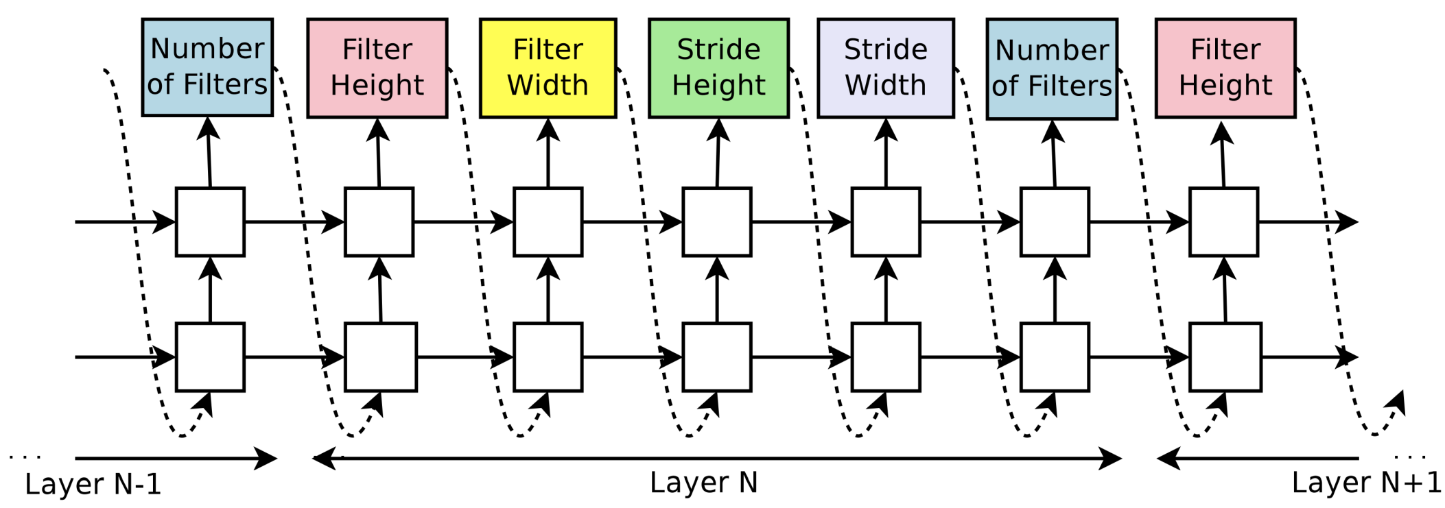
This process can be viewed as reinforcement learning:
The list of tokens that the controller predicts can be viewed as a list of actions $a_{1∶T}$ to design an architecture for a child network and the valid accuracy of a given dataset is the feedback $R$.
The goal of the controller is to maximize its expected reward $J(\theta_c)$.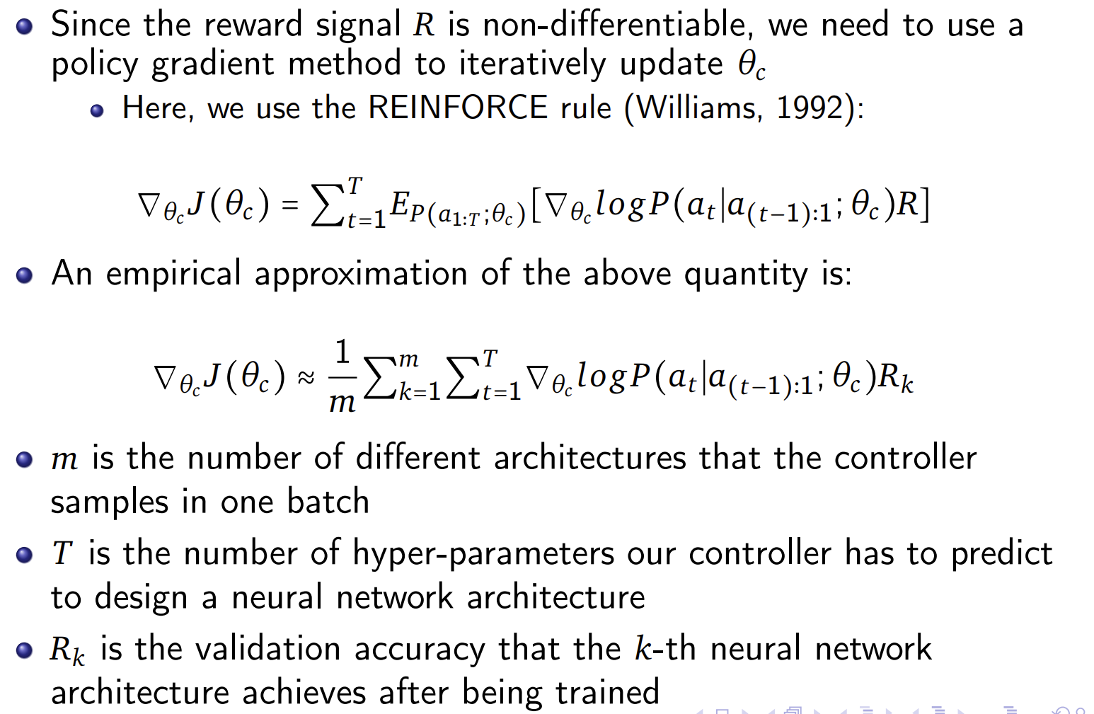
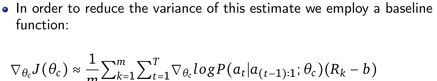
The baseline b is an exponential moving average of the previous architecture accuracies and does not depend on the current action. (Similar to Adam)
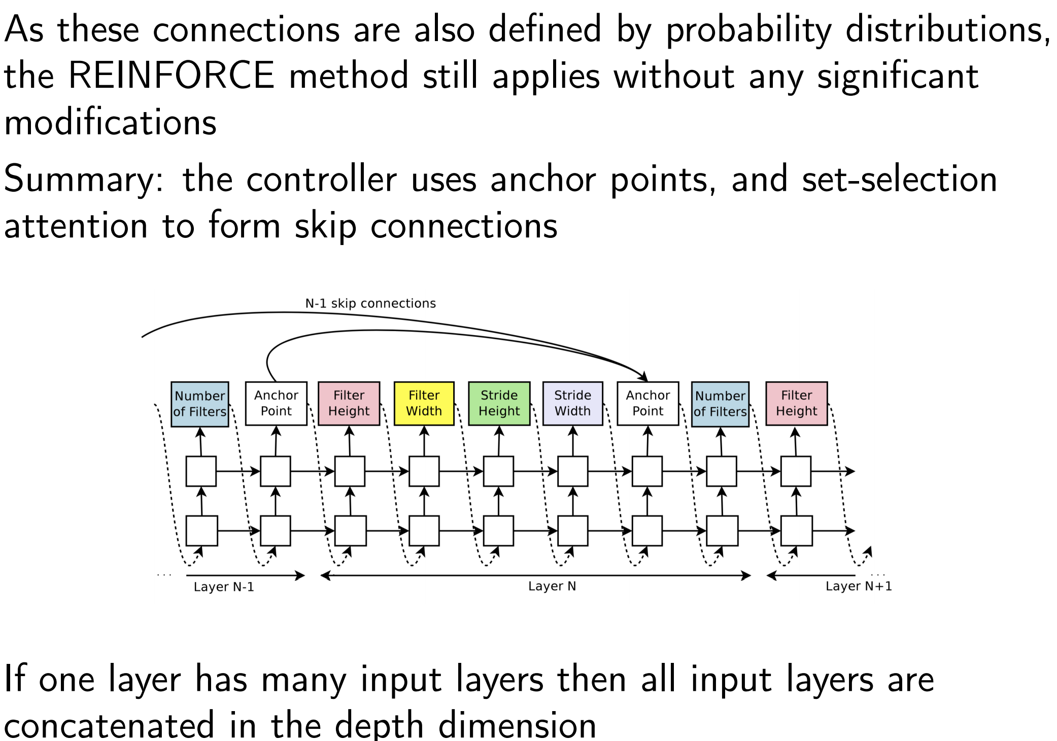
Generate architecture with Skip Connections
Set-selection type attention
At layer N, we add an anchor point which has N − 1 content-based sigmoids to indicate the previous layers that need to be connected.
Each sigmoid is a function of current hidden-state of the controller and previous hidden-states of the previous N − 1 anchor points.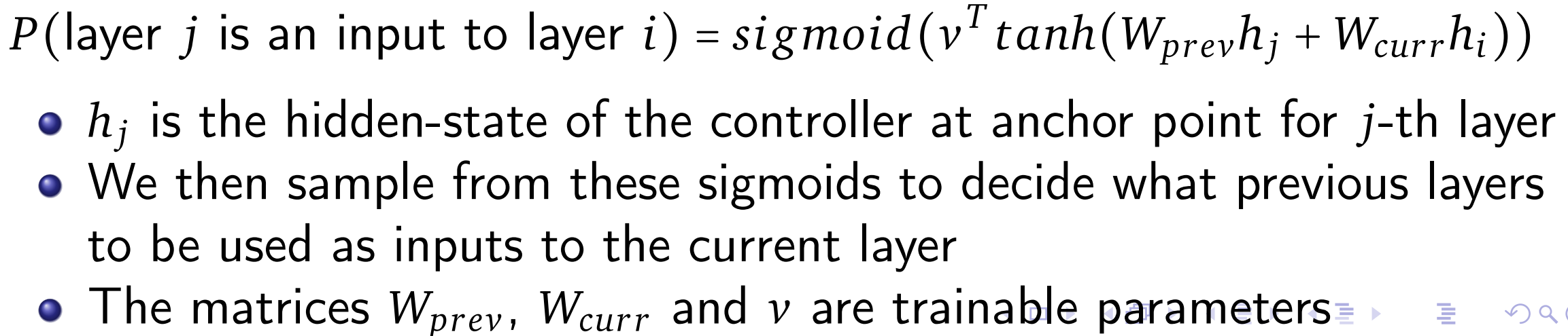
Failures:
- One layer is not compatible with another layer
- One layer may not have any input or output
Solutions:
- Pad the smaller layer with zeros.
- If no input layer, take the original data as input.
- Concat all the layers where output is not connected and send this hidden state to the classifier.
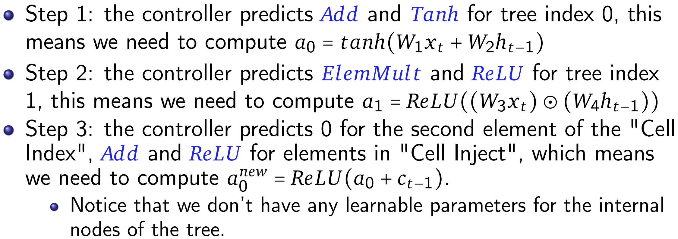
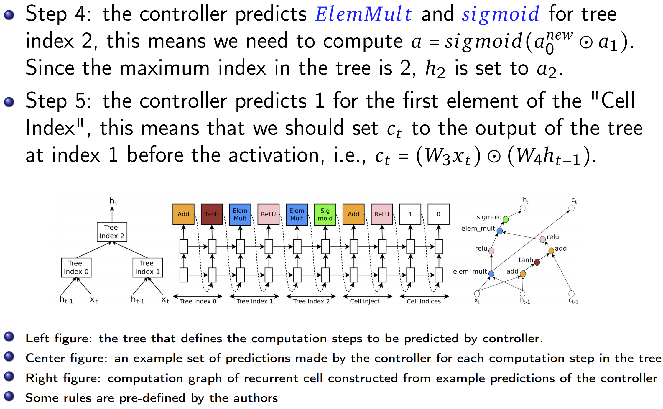
Generate RNN using RNN
Experiment
In experiments of autoML, we still need human knowledge such as the filter height, number of filters and initialazition of parameters to design the model.
Reward for updating the contoller is the maximum validation accuracy of the last 5 epochs(total 50) of one generated model.
CNN for Cifar10
Accuracy by human of denseNet is a little higher than NAS. We wish to minimize the parameters to make the model cheap enough to set into a mobile device. NAS can generate small models with reasonable accuracy.
RNN for Penn Tree-Bank dataset
LR for controller is 0.0005.
The number of input pairs to the RNN cell is called the “base number“ and set to 8 in our experiments(much more complex than 2 in the above example).
Every child model is constructed and trained for 35 epochs.
Every child model has two layers, with the number of hidden units adjusted so that total number of learnable parameters roughly match the “medium” baselines.
The reward function is $\frac{c}{(validation\quad perplexity)^2}$.
When the base number is 8, the search space has approximately $6×10^{16}$ architectures, it is too expensive to search them all.
Goal: keep a medium size model
NAS works well in this task to have both less parameters and lower test perplexity.
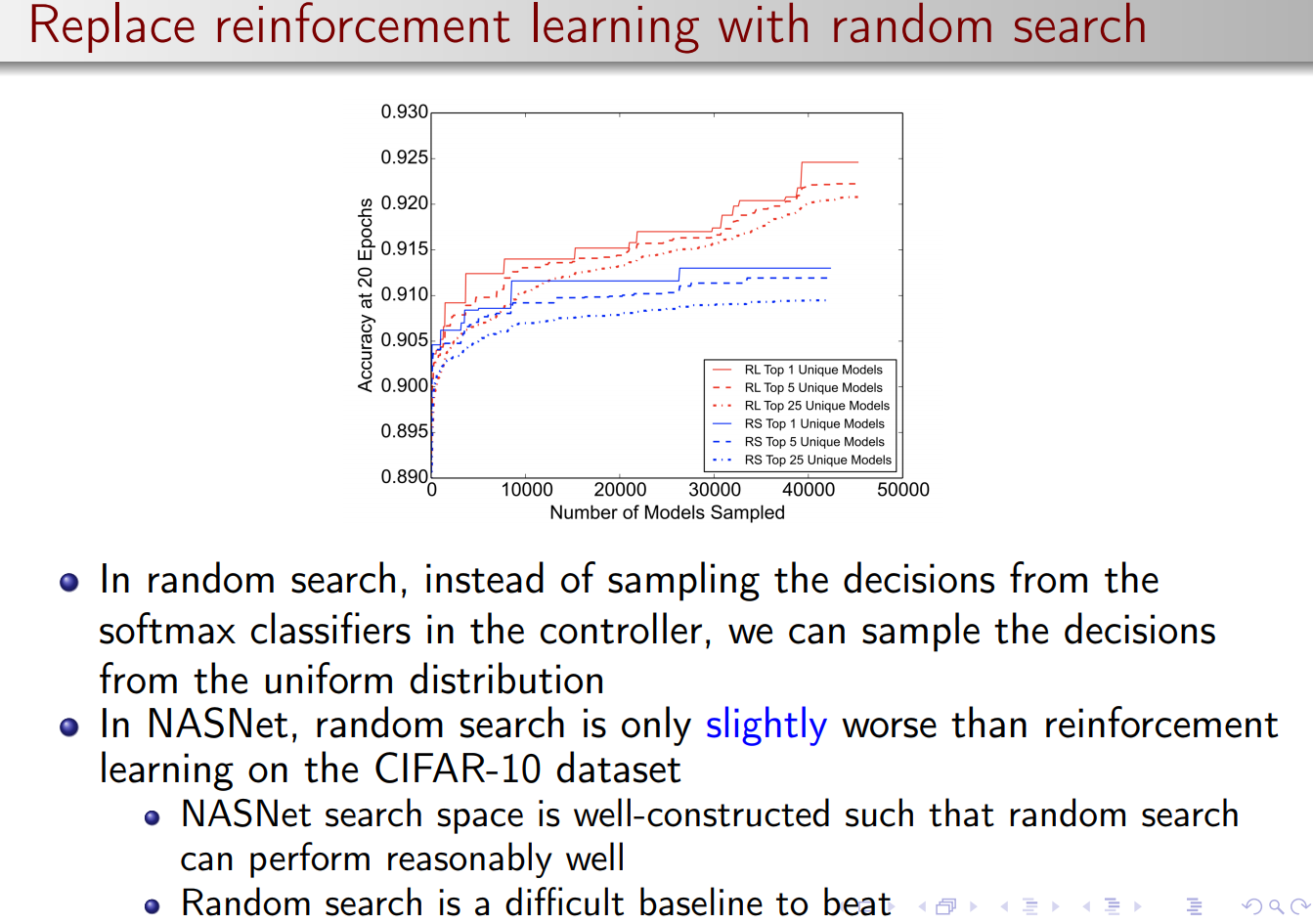
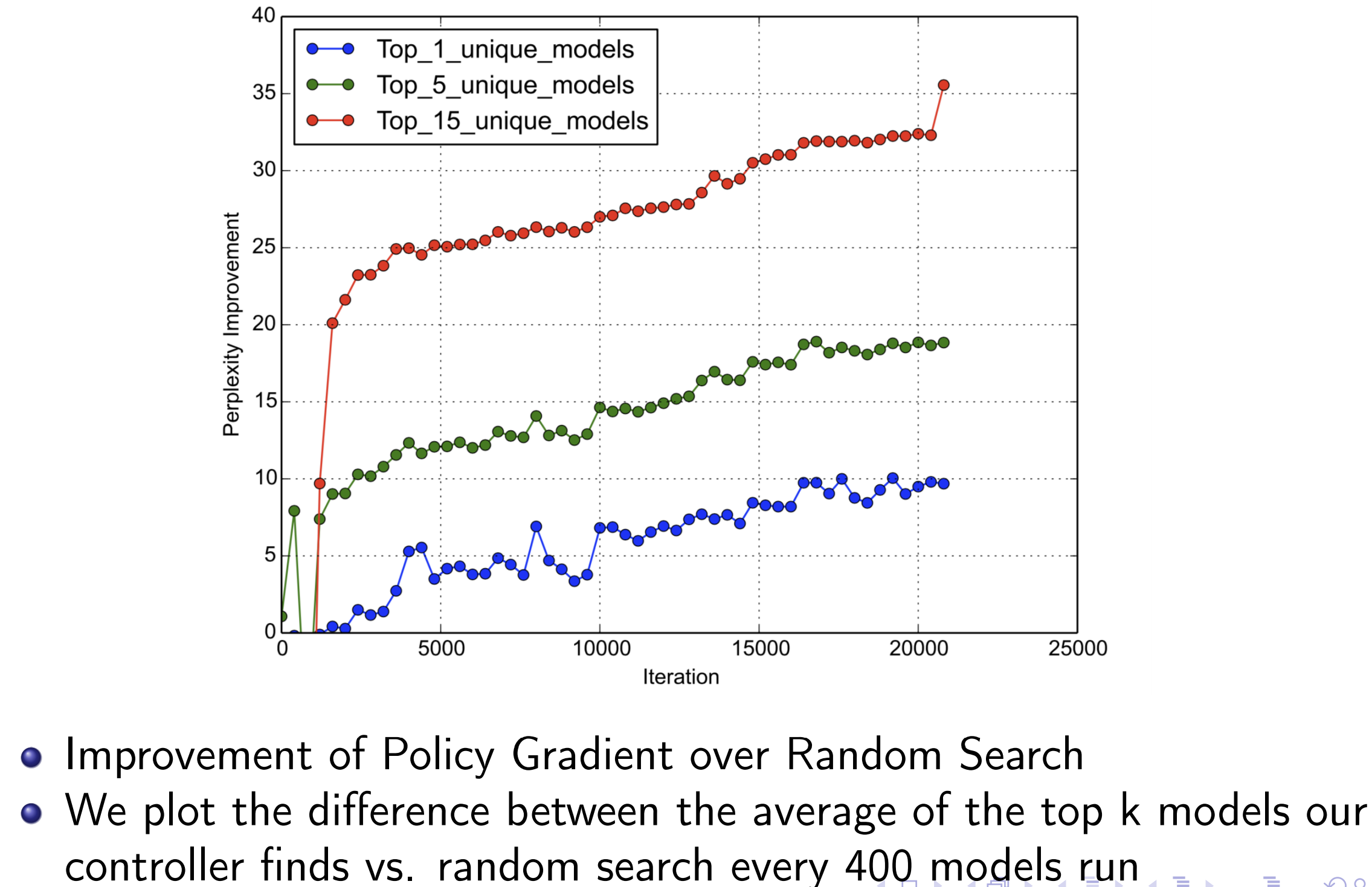
Policy Gradient vs Random Search
NASNet: searching a cell rather than an architecture
Limitations of vanilla NAS:
- Computationally expensive even for small datasets (e.g. Cifar-10)
- No transferable between datasets (from small to large?)
People observe that successful models are repeating special patterns. So instead of searching the whole architecture, we can search for efficient patterns.
Concepts and Method
It may be possible for the controller to predict a general convolutional cell expressed in terms of motifs. The cell can then be stacked in series to handle inputs of arbitrary spatial dimensions and filter depth.
The overall architectures of the convolutional nets are manually predetermined.
- They are composed of convolutional cells repeated many times
- Each cell has the same architecture, but different weights
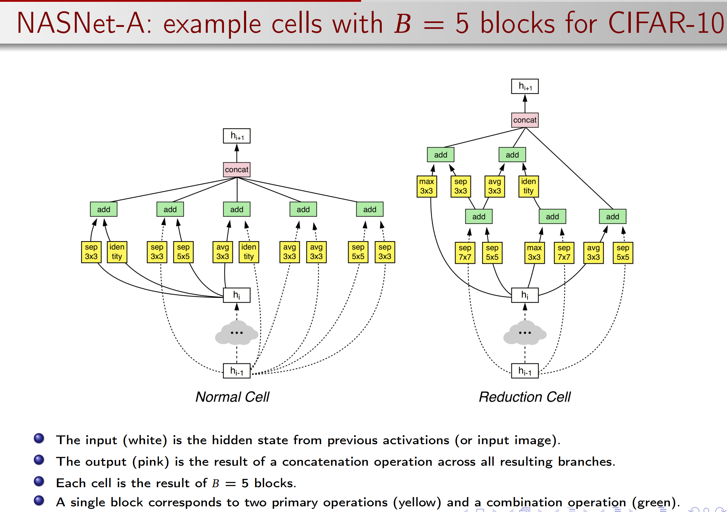
Two type of cells to easily build scalable architectures for images of any size:
Normal Cell: returning a feature map of the same dimension.
Reduction Cell: returning a feature map where the feature map’s
height and width is reduced by a factor of two.
Researchers empirically found it beneficial to learn two separate architectures for normal cell and reduction cell.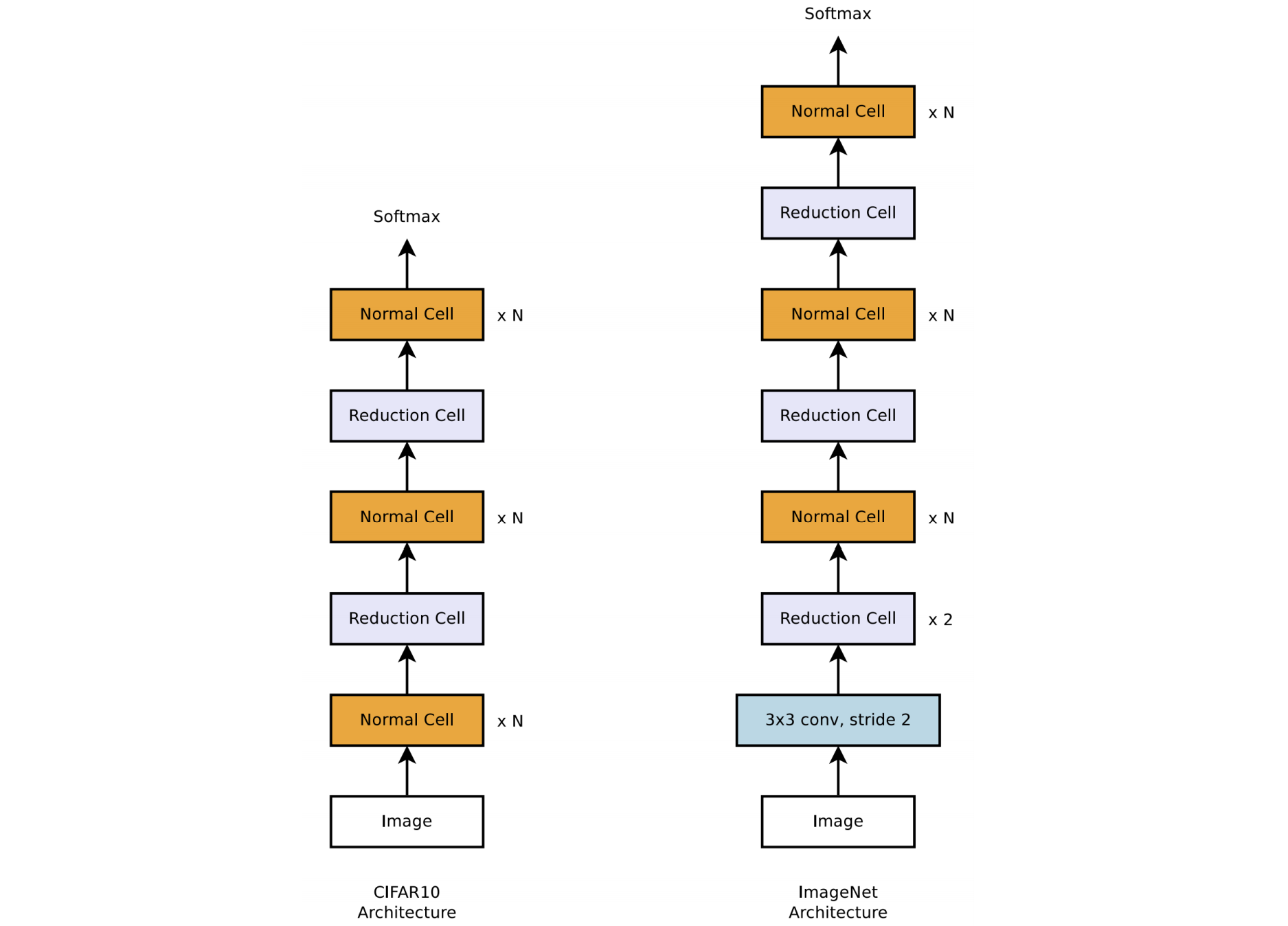
We use a common heuristic to double the number of filters in the output whenever the spatial activation size is reduced in order to maintain roughly constant hidden state dimension.
We consider the number of motif repeating times N and the number of initial convolutional filters as free parameters.
Now the question is: how to use a controller to generate a block of a cell.
So we first build a block, and combine several blocks as a cell, then use the cell to build the architecture.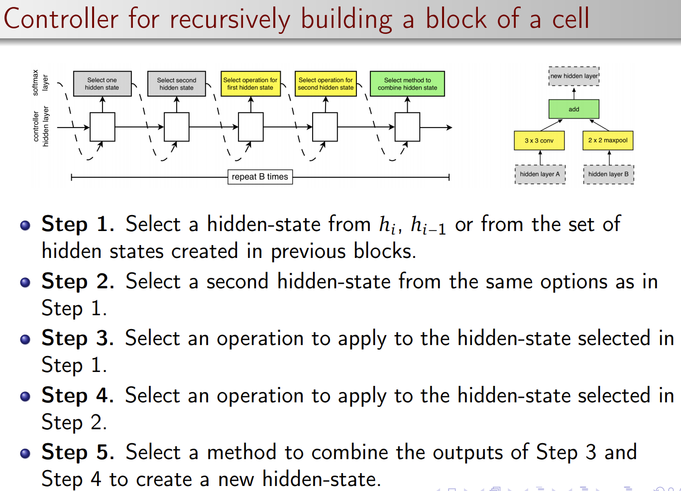
To allow the controller to predict both Normal Cell and Reduction Cell, we simply make the controller have 2 × 5B predictions in total.
The first 5B predictions are for the Normal Cell and the second 5B predictions are for the Reduction Cell.
Experimental Results