Generative Adversarial Networks

Introduction to GANs

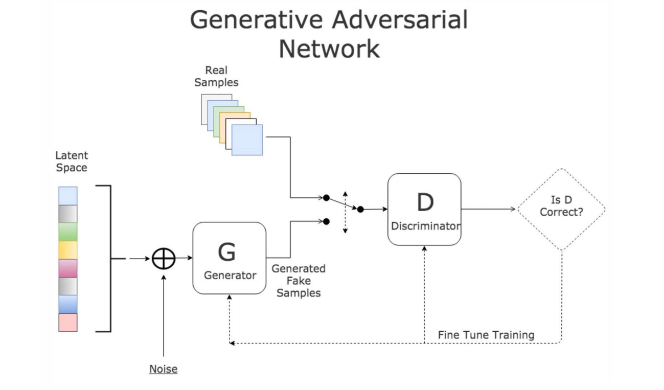
Discriminator learns from real dataset and make judgement of input data.
Generator uses noise vestor to generate fake data and feed into discriminator, based on the feedback it can generate better samples.

• Deep Convolutional GAN can train stable GANs at scale.
• BigGan can generate synthetic photos that are practically indistinguishable.
• Generate faces of anime characters.
• Image-to-Image Translation: transfer from daytime to nighttime; sketcher to color.
• Text-to-Image: generate plausible photos from textual descriptions of simple objects.
• Semantic-Image-to-Photo: given a semantic image or sketch as input.
• Face Frontal View Generation: given photos taken at an angle.
• Photos to Emojis: translate images from one domain to another.
• Photograph Editing: reconstruct photos of faces with specific specified features.
• Face Aging: generate photos of faces with different apparent ages.
• Photo Blending: blend elements from different photos.
• Super Resolution: generate pictures with higher pixel resolution.
• Photo Inpainting: filling in an area of a photo that was removed.
• Clothing Translation: input someone with a cloth on and output the cloth in catalog
• Video Preodiction: predict videos given a single static image (ambiguous task)

Training of GANs

Two neural networks contest with each other in a zero-sum game.
The goal of generator is to fool the discriminator but not to imitate a specific image.
This enables the model to learn in an unsupervised manner(no specific target).
Unsupervised: learn the distribution function $p(x,y)$ to generate synthetic $x’$ and $y’$.
Supervised: model the conditional probability distriburion function(p.d.f) $p(y|x)$.

Other generative models:

• Variational Autoencoders(VAEs)
• pixelCNN / pixelRNN
• real NVP

GANs are popular because it can generate high dimensional data.
Generative models can be viewed as containing more information than discriminative models and they are also used for discriminative tasks like classification.

Generative Adversarial Networks are composed of two models:

• Generator $G(z,\theta_1)$: aims to generate new data similar to the expected one, maps input noise variables $z$ to the desired data space $x$.
  Goal: Maximize $D(G(z))$
• Discriminator $D(x,\theta_2)$: recognizes if an input data is real by outputing the probability that the data comes from the real dataset.
  Goal: Maximize $D(x)$ and minimize $D(G(z))$

The competition between these two models is what improves their knowledge until Generator succeeds in creating realistic data.
In practice we use a log loss instead of the raw probability.

Discriminator and Generator are trying to optimize the opposite loss function: two agents playing a minimax game with value function $V(G,D)$:

$$\min_G \max_D V(D,G) = \mathbb{E}_{x\sim p_{data} (x)}[logD(x)]+\mathbb{E}_{z\sim p_z(z)}[log(1-D(G(z)))]$$

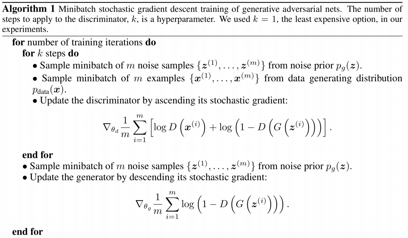
The fundamental steps to train a GAN:

1. Sample a noise set and a real-data set, each with size m
2. Train the Discriminator on this data batch for several steps
3. Sample a different noise subset with size m
4. Train the Generator on this data batch
5. Repeat from Step 1

DC-GAN, Conditional GAN, and W-GAN

Deep Convolutional Generative Adversarial Networks

1. Use strided convolutions instead of deterministic spatial pooling functions(eg. max pooling), so the Discriminator can learn its own spatial downsampling and Generator can learn its own spatial upsampling.
2. Eliminate fully connected layers on top of convolutional features.
3. Batch Normalization helps gradients flow in deeper models, not applied to Generator’s output layer and Discriminator’s input layer to avoid sample oscillation and model instability.
4. Generator uses ReLU for all layers except for output which uses Tanh,
   Discriminator uses LeakyReLU for all layers.

Generator: No fully connected or pooling layers are used.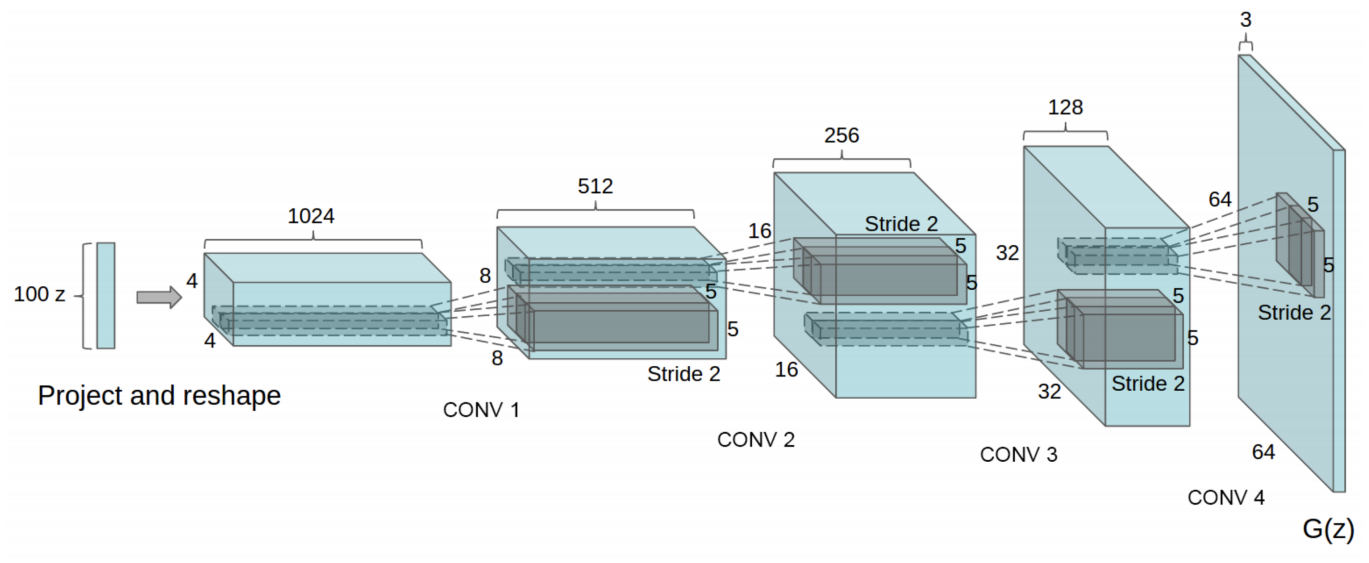

Discriminator is like an inverse of Generator.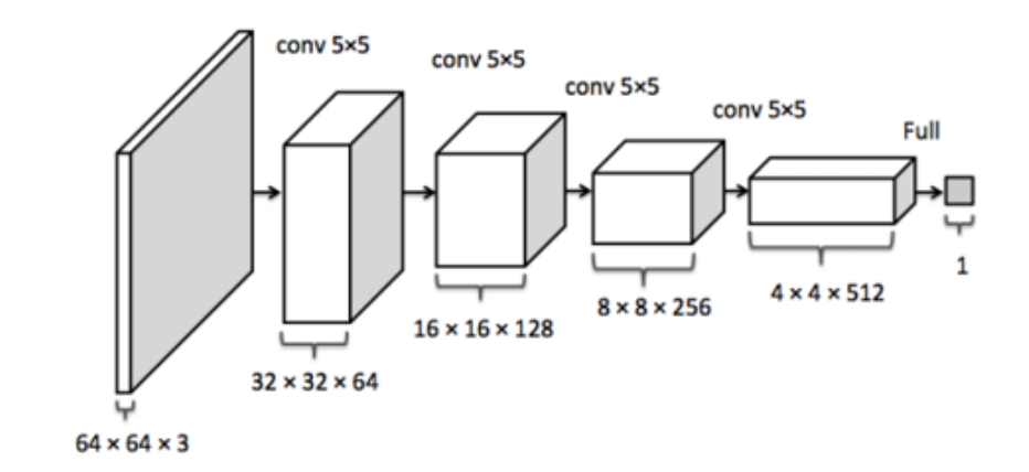

Conditional GANs

Generators is trained to generate examples from the input domain(conditions), so its input is combined with some additional input(eg. a class value).
Discriminator is also conditioned and its input image is combined with an additional input.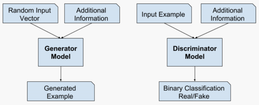

The conditional domain allows for applications such as text-to-image or image-to-image.
We can perform conditioning by feeding the extra information $y$ into both the discriminator and generator as additional input layer:

$$\min_G \max_D V(D,G) = \mathbb{E}_{x\sim p_{data} (x)}[logD(x|y)]+\mathbb{E}_{z\sim p_z(z)}[log(1-D(G(z|y)))]$$

If the generator ignores the input conditions, the discriminator will give them a low score even though the input image is realistic.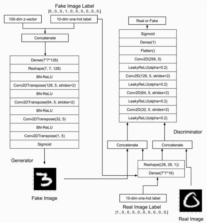

Wasserstein GAN (WGAN)

WGAN uses a critic that scores the realness or fakeness of a given image to replace the discriminator who predicts the probability as being real or fake.

The benefit is that the training process is more stable and less sensitive to model architecture and choice of hyperparameter and the loss of the discriminator appears to relate to the quality of images created by the generator.

The Wasserstein Distance is the minimum cost of transporting mass in converting the real data distribution $r$ to generated data distribution $g$ , which is defined as the greatest lower bound(infimum) for any transport plan(i.e. the cost of the cheapest plan):

$$W(\mathbb{P}_r,\mathbb{P}_g)=\inf_{\gamma\in\prod(\mathbb{P}_r,\mathbb{P}_g)}\mathbb{E}_{(x,y)}[||x-y||]$$

Using Kantorovich-Rubinstein duality, we can simplify it to:

$$W(\mathbb{P}_r,\mathbb{P}_\theta)=\sup_{||f||_L\leq 1} \mathbb{E}_{x\sim \mathbb{P}_r}[f(x)] - \mathbb{E}_{x\sim \mathbb{P}_\theta}[f(x)]$$

$sup$ is the least upper bound and $f$ is a 1-Lipschitz function which means:

$$|f(x_1)-f(x_2)|\leq |x_1-x_2|$$

so that the minimum $|f(x_1)-f(x_2)|$ correspond to the minimum $|x_1-x_2|$ .
We can build a deep network to learn the 1-Lipschitz function. The network is similar to discriminator, just without the sigmoid function and output a score to show how real the input images are rather than a probability.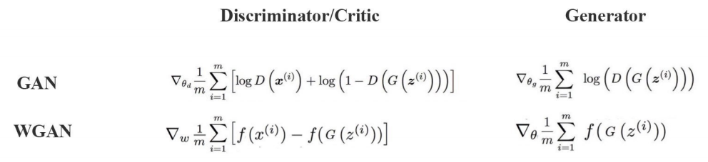

$f$ has to be a 1-Lipschitz function. To enforce the constraint, WGAN applies a very simple clipping to restrict the maximum weight value in $f$ , i.e. the weights of the discriminator must be within a certain range controlled by the hyperparameters $c$.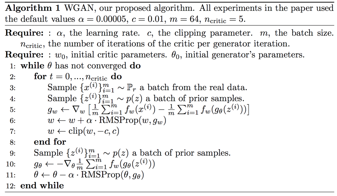

GAN’s loss measures how well it fools the discriminator, while WGAN’s loss function reflects the image quality which is more desirable.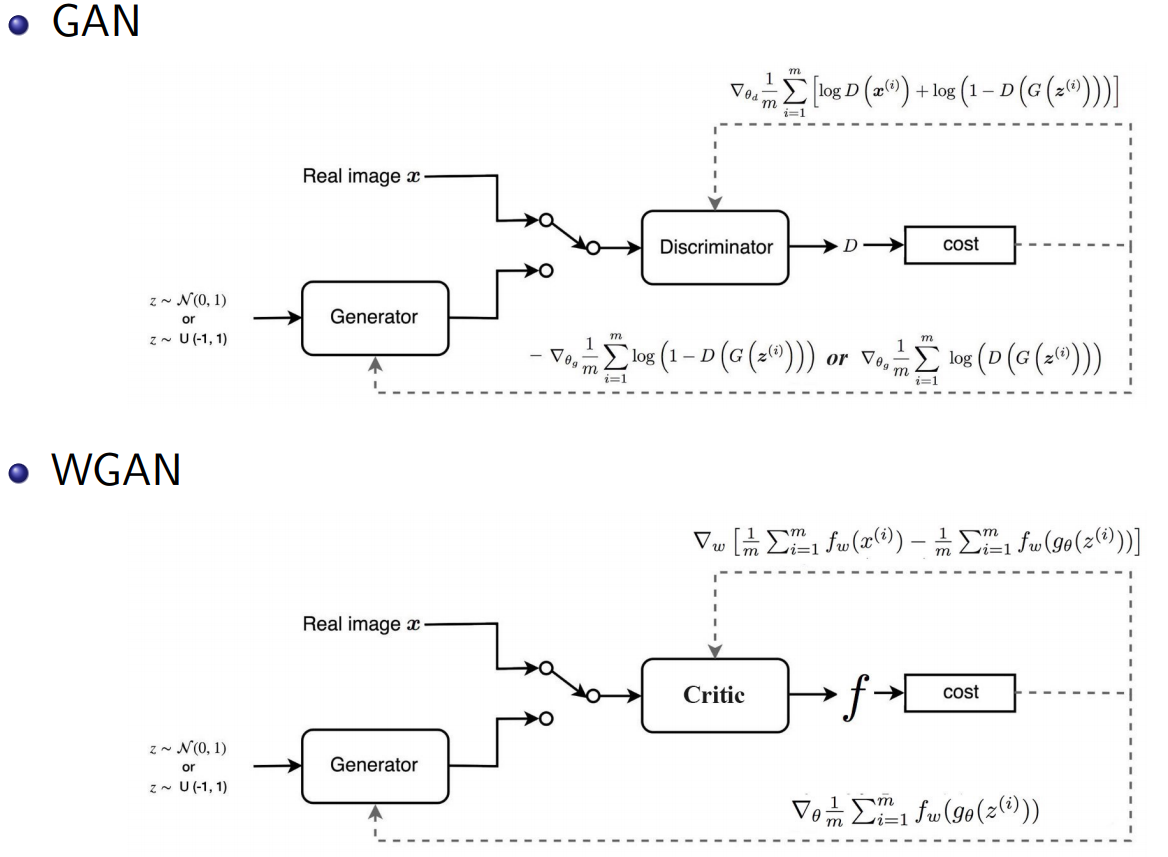

WGAN is more stable as it can perform without batch normalization but GANs without BN collapse.