NNDL Summary

Linear Regression

Linear regression

Univariate: single feature $x\in R$
Multivariate: multiple features $\boldsymbol{x}\in R^m$
Linear Transformation: $\widetilde{y}=\boldsymbol{w^Tx}$
Loss: measures the difference between the prediction and the ground truth
Training: to optimize(i.e. minimize) the loss w.r.t parameters($\boldsymbol{w}$)

Gradient descent algorithm

minimize the target loss iterately, for each iteration:
conpute the gradient of average loss

• for single feature multiple examples: $$J(w)=\frac{1}{2m}\sum_{i=1}^m(wx^{(i)}-y^{(i)})^2$$
• for multiple features one single instance: $$J(\boldsymbol{w})=\frac{1}{2}(\boldsymbol{w^Tx}-y)^2$$
• for multiple features multiple examples: $$J(\boldsymbol{w})=\frac{1}{2m}(\mathbf{X}\boldsymbol{w}-\boldsymbol{y})^T(\mathbf{X}\boldsymbol{w}-\boldsymbol{y})$$

update parameter in the opposite of the gradient direction: $\boldsymbol{w}=\boldsymbol{w}-\alpha\frac{\partial J}{\partial \boldsymbol{w}}$

• for single feature multiple examples: $$\frac{\partial J}{\partial w}=\sum_{i=1}^m(wx^{(i)}-y^{(i)})$$
• for multiple features one single instance: $$\frac{\partial J}{\partial \boldsymbol{w}}=(\boldsymbol{w^Tx}-y)\boldsymbol{x}$$
• for multiple features multiple examples: $$\frac{\partial J}{\partial \boldsymbol{w}}=\frac{1}{m}\mathbf{X}^T(\mathbf{X}\boldsymbol{w}-\boldsymbol{y})$$

stop until paremeters converge or reach a certain number of iterations.

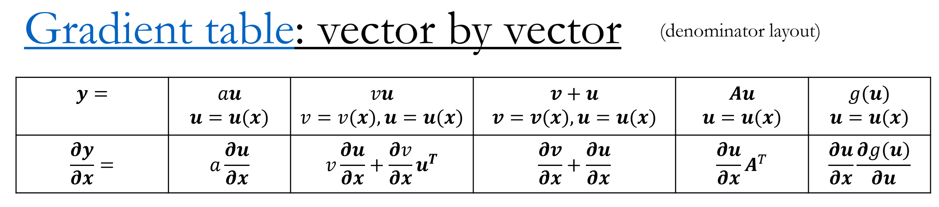
• $f(x)=g(x)+h(x)\quad\to\quad f’(x)=g’(x)+h’(x)$
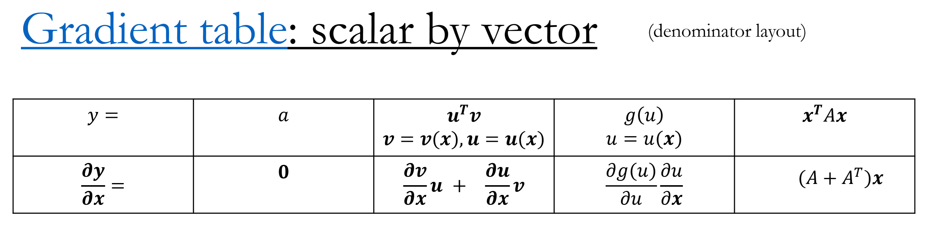
• $f(x)=g(x)h(x)\quad\to\quad f’(x)=g’(x)h(x)+g(x)h’(x)$
• $f(x)=\frac{g(x)}{h(x)}\quad\to\quad f’(x)=\frac{g’(x)h(x)-g(x)h’(x)}{h(x)^2}$
• $f(x)=g(u),g(u)=h(x)\quad\to\quad f’(x)=g’(u)h’(x)$

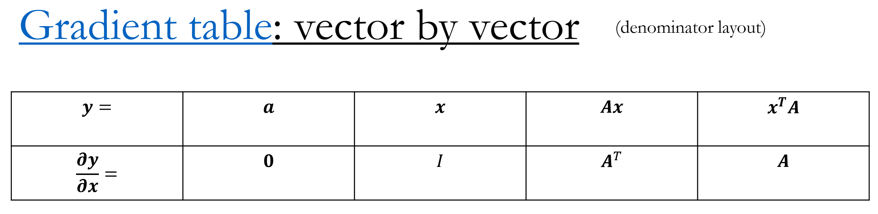
Example:
$y=(\mathbf{A}\boldsymbol{x})^T(2\boldsymbol{x+z})$ , $\mathbf{A}$ is a square matrix, $\boldsymbol{x}$ and $\boldsymbol{z}$ are vectors, y is a scalar, what is $\frac{\partial y}{\partial \boldsymbol{x}}$ ?

$$\boldsymbol{u}=\mathbf{A}\boldsymbol{x}\quad \boldsymbol{v}=2\boldsymbol{x+z}$$ $$\begin{aligned}\frac{\partial y}{\partial \boldsymbol{x}}&=\frac{\partial \boldsymbol{u^Tv}}{\partial \boldsymbol{x}}=\frac{\partial \boldsymbol{u}}{\partial \boldsymbol{x}}\cdot\boldsymbol{v}+\frac{\partial \boldsymbol{v}}{\partial \boldsymbol{x}}\cdot\boldsymbol{u}\\&=\mathbf{A}^T(2\boldsymbol{x+z})+(2\boldsymbol{I})\cdot(\mathbf{A}\boldsymbol{x})\\&=2\mathbf{A}^T\boldsymbol{x}+\mathbf{A}^T\boldsymbol{z}+2\mathbf{A}\boldsymbol{x}\end{aligned}$$

$L=\frac{1}{2}(\boldsymbol{w^Tx}-y)^2$, $\boldsymbol{x}=(1,2)^T$, $\boldsymbol{w}=(2,1)^T$, $y=0$, compute the gradient of $\frac{\partial L}{\partial \boldsymbol{w}}$

$$\begin{aligned}\frac{\partial L}{\partial \boldsymbol{w}}&=(\boldsymbol{w^Tx}-y)\boldsymbol{x}\\&=(\begin{pmatrix}2,1\end{pmatrix}\cdot\begin{pmatrix}1\\2\end{pmatrix}-0)\cdot\begin{pmatrix}1\\2\end{pmatrix}\\&=(4-0)\cdot\begin{pmatrix}1\\2\end{pmatrix}\\&=\begin{pmatrix}4\\8\end{pmatrix}\end{aligned}$$

Classification

Logistic regression

From Linear regression to Logistic regression:
The function $\widetilde{y}=\begin{cases} 1,\qquad\qquad if\boldsymbol{w^Tx}>0 \\ 0,\qquad\qquad else\end{cases}$ is not differentiable, therefore we use Logistic function as the probability: $p=\sigma (z) = \sigma(\boldsymbol{w^Tx})=\frac{1}{1+e^{-\boldsymbol{w^Tx}}}$
$L2$ loss function: $L=\frac{1}{2}||p-y||^2=\frac{1}{2}||\sigma(z)-y||^2$
thus the gradient is: $\frac{\partial L}{\partial \boldsymbol{w}}=(\sigma(z)-y)\sigma(z)(1-\sigma(z))\boldsymbol{x}$
There exists gradient vanishing. In order to solve this problem, we use the binary cross entropy to compute the loss: $L=-ylogp-(1-y)log(1-p)$
The gradient now is : $\frac{\partial L}{\partial \boldsymbol{w}}=(p-y)\boldsymbol{x}$

$$z=\boldsymbol{w^Tx},\boldsymbol{x}\in R^{n\times 1}, \boldsymbol{w}\in R^{n\times 1}$$ $$p=\sigma (z)=\frac{1}{1+e^{-z}}$$ $$L(p, y)=-ylogp-(1-y)log(1-p)$$ $$\frac{\partial L}{\partial \boldsymbol{w}}=(p-y)\boldsymbol{x}$$

Multi-label classification

对第 $i$ 个类别有：
$z_i=\boldsymbol{W}_i\boldsymbol{x}+b_i\quad p_i=\sigma(z_i)\quad L_{ce}=-y_ilogp_i-(1-y_i)log(1-p_i)$
对于所有类别向量化表示为:
$\boldsymbol{z}=\boldsymbol{W}\boldsymbol{x}+\boldsymbol{b}\quad \boldsymbol{p}=\sigma(\boldsymbol{z})\quad L_{ce}=-\boldsymbol{y}^Tlog\boldsymbol{p}-(1-\boldsymbol{y})^Tlog(1-\boldsymbol{p})$

Softmax/multinomial classification

Multi-class single-label: classes are not independent, they are exclusive.

• Softmax function $$p_i=\frac{e^{z_i}}{\sum_j e^{z_j}}=softmax(z_i)$$
• Cross-entropy loss $$L_{ce}(\boldsymbol{x},\boldsymbol{y})=\sum_i-y_ilogp_i=-\boldsymbol{y}^Tlog\boldsymbol{p}$$ $$\frac{\partial J}{\partial \mathbf{W}}=\frac{1}{m}(\mathbf{P}-\mathbf{Y})\mathbf{X}^T\in R^{k\times n}, \mathbf{X}\in R^{(m\times n)} ,\mathbf{Y}\in R^{(m\times k)}$$

Detail:
$L=\frac{1}{2}(\sigma(\boldsymbol{w^Tx})-y)^2$

$$z=\boldsymbol{w^Tx}$$ $$\begin{aligned}\frac{\partial L}{\partial \boldsymbol{w}}&=(\sigma(z)-y)\frac{\partial \sigma(z)}{\partial z}\frac{\partial z}{\boldsymbol{w}}\\&=(\sigma(z)-y)\frac{\partial (1-e^{-z})^{-1}}{\partial z}\boldsymbol{x}\\&=(\sigma(z)-y)(-1(1-e^{-z})^{-2})\frac{\partial (1-e^{-z})}{\partial z}\boldsymbol{x}\\&=(\sigma(z)-y)(-\sigma(z)^2)\frac{\partial (1-e^{-z})}{\partial z}\boldsymbol{x}\\&=(\sigma(z)-y)(-\sigma(z)^2)e^{-z}\boldsymbol{x}\\&=(\sigma(z)-y)(-\sigma(z)^2)(1-\frac{1}{\sigma(z)})\boldsymbol{x}\\&=(\sigma(z)-y)(-\sigma(z))(\sigma(z)-1)\boldsymbol{x}\\&=(\sigma(z)-y)\sigma(z)(1-\sigma(z))\boldsymbol{x}\end{aligned}$$

$L_{ce}=-ylogp-(1-y)log(1-p)\quad p=\sigma(z)$

$$\begin{aligned}\frac{\partial L}{\partial \boldsymbol{w}}&=\frac{\partial L}{\partial p}\frac{\partial p}{\partial z}\frac{\partial z}{\partial \boldsymbol{w}}\\&=(-\frac{y}{p}+\frac{1-y}{1-p})p(1-p)\boldsymbol{x}\\&=(-y+py+p-py)\boldsymbol{x}\\&=(p-y)\boldsymbol{x}\end{aligned}$$

$L_{ce}(\boldsymbol{x},\boldsymbol{y})=\sum_i-y_ilogp_i=-\boldsymbol{y^T}log\boldsymbol{p}$

$$\frac{\partial J}{\partial \mathbf{W}}=\frac{1}{m}(\mathbf{P}-\mathbf{Y})\mathbf{X}^T\in R^{k\times n}$$ $$\mathbf{X}\in R^{(m\times n)} ,\mathbf{Y}\in R^{(m\times k)}$$

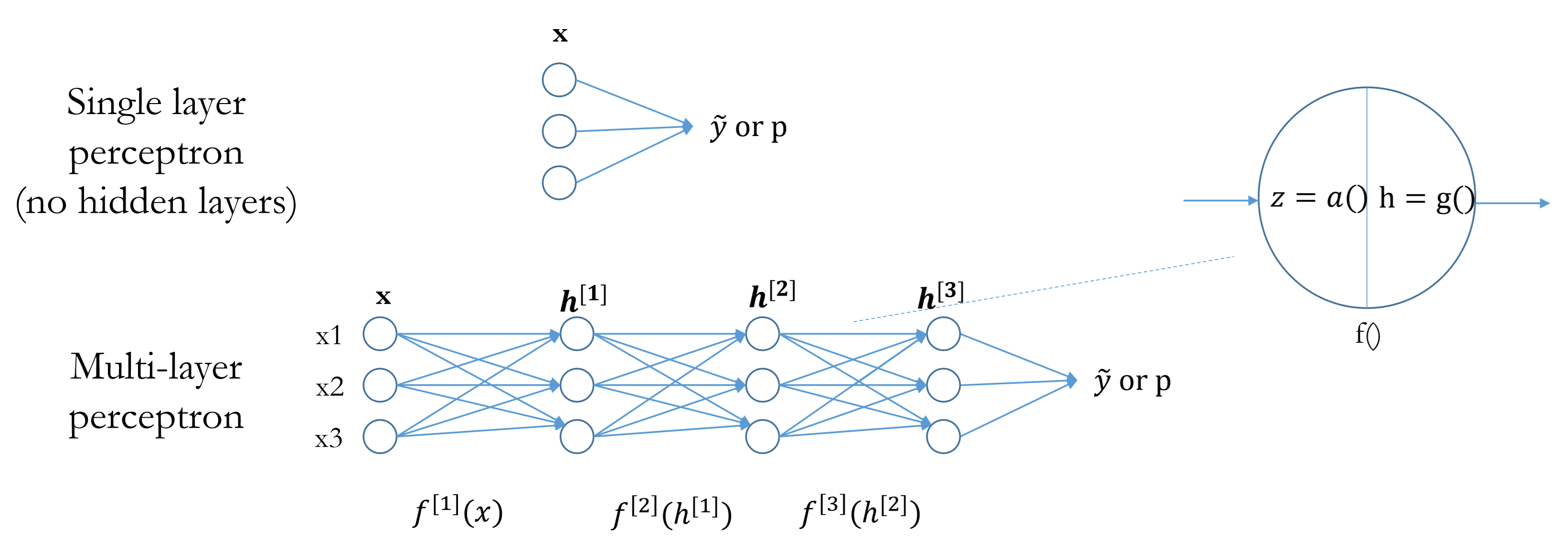
From Shallow to Deep Neural Network

MLP

A net with multiple layers that transform input features into hidden features and then make predictions .

• At least one non-linear hidden layer
• A linear function is always followed by a non-linear function

$$\boldsymbol{z}^{[i]}=a^{[i]}(\boldsymbol{h}^{[i-1]})=W^{[i]}\boldsymbol{h}^{[i-1]}+\boldsymbol{b}^{[i]}$$ $$W^{[i]}\in R^{n_i\times n_{i-1}}\quad \boldsymbol{b}^{[i]}\in R^{n_i}$$

Chain Rule

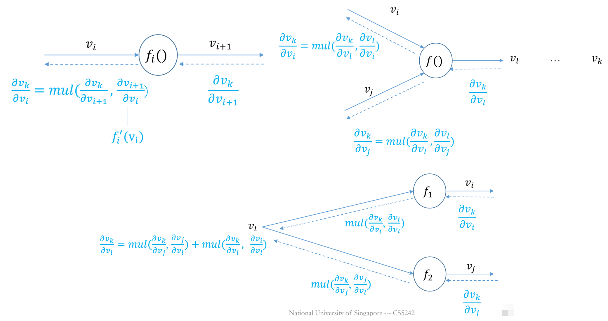
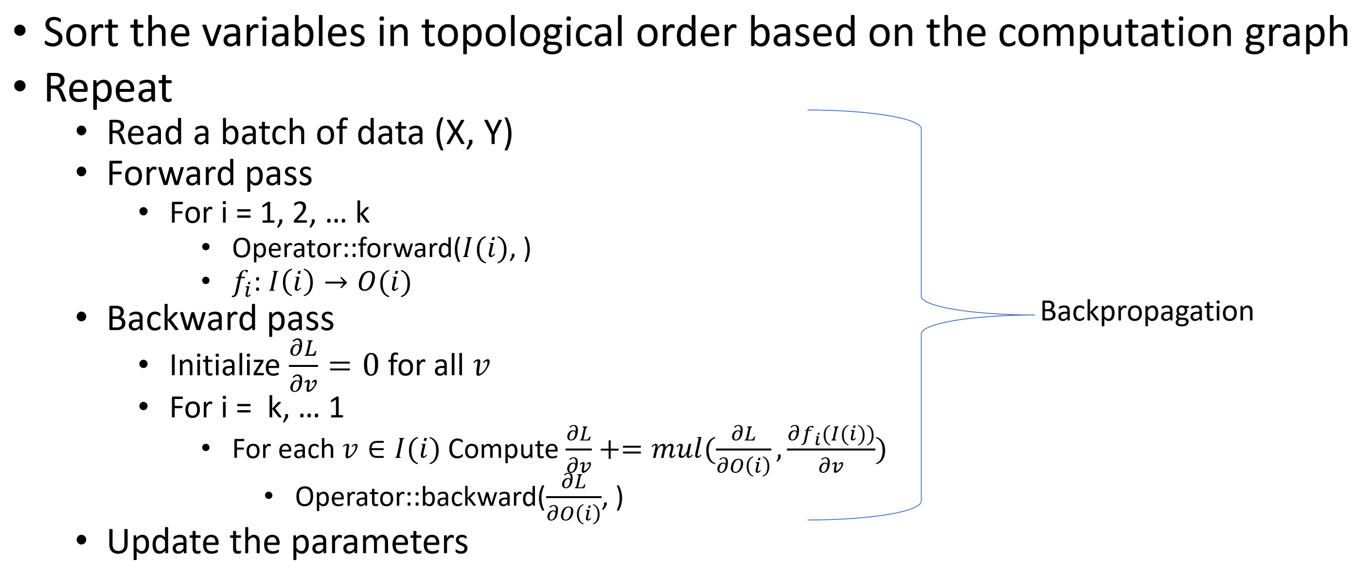
Backpropagation

• Add bias
  $\boldsymbol{A}\in R^{m\times n}\quad b\in R^{1\times n}$
  Forward($\boldsymbol{A},b$): $\boldsymbol{C}=\boldsymbol{A}+b$
  Backward($d\boldsymbol{C},\boldsymbol{A},b$): $d\boldsymbol{A}=d\boldsymbol{C}\quad db=1^Td\boldsymbol{C}$

• Array and scalar multiplication
  $\boldsymbol{v}$ is an array, $k$ is a scalar(usually hyperparameter)
  Forward($\boldsymbol{v},k$): $\boldsymbol{c}=k\boldsymbol{v}$
  Backward($d\boldsymbol{c},\boldsymbol{v},k$): $d\boldsymbol{v}=kd\boldsymbol{c}$

• Matmul matrix multiplication operation
  $\boldsymbol{A}\in R^{m\times k}\quad \boldsymbol{B}\in R^{k\times n}$ (including matrix with a single column or row)
  Forward($\boldsymbol{A},\boldsymbol{B}$):$\boldsymbol{C=A\cdot B^T}\in R^{m\times n}$
  Backward($d\boldsymbol{C},\boldsymbol{A},\boldsymbol{B}$): $d\boldsymbol{A}=d\boldsymbol{C}\cdot \boldsymbol{B^T}\quad d\boldsymbol{B}=\boldsymbol{A^T}\cdot d\boldsymbol{C}$

• Logistic operation
  $a$ is an array of any shape
  Forward($a$): $b=\sigma(a)$
  Backward($db,a$): $da=db\times b\times (1-b)$

• Softmax-Cross-entropy operation
  Forward($\boldsymbol{Z},\boldsymbol{P}$): $\boldsymbol{P}=softmax(\boldsymbol{Z})\quad L=\frac{1}{m}sum(-YlogP) $
  Backward($\boldsymbol{Z},\boldsymbol{P}$): $d\boldsymbol{Z}=\frac{1}{m}(\boldsymbol{P}-\boldsymbol{Y})$

Training Deep Networks

Mini-batch stochastic gradient descent (SGD)

• Reduces the chance of local optimal points and saddle points from GD
• More stable and smooth than standard SGD
• Extensions: Momentum, RMSProp, Adam

• Smooth the gradients by preserving historical gradients
• Adaptive learning rate per parameter

Momentum:

$$v=\beta v+\alpha g$$ $$w=w-v$$

RMSprop:

$$s=\beta s+(1-\beta)g^2\qquad moving\quad average$$ $$w=w-\frac{\alpha}{\sqrt{s+\epsilon}}g\qquad nomalize\quad the\quad gradient$$

Adam:

$$v=\beta_1 v+(1-\beta_1)g\quad \hat v = \frac{v}{1-\beta_1^t}$$ $$s=\beta_2 s+(1-\beta_2)g^2\quad \hat s = \frac{s}{1-\beta_2^t}$$ $$w=w-\frac{\alpha}{\sqrt{s+\epsilon}} v=w-\frac{\alpha}{\sqrt{\hat s+\epsilon}}\hat v$$

Tricks

• Learning rate decay: start large and decrease gradually
• Randomly initialize parameters: break symmetry
  and avoid gradient vanishing / exploding
• Data normalization

Overfitting and underfitting

• Underfitting means high bias, Overfitting means high variance.
• Regularization: Early stop and L2 Norm.
• Model capacity: the ability for the model to fit different functions or datasets; with more unconstrained parameters, the model can fit more functions and datasets.
• Hyper-parameter tuning:
  • Tune parameters using training data.
  • Tune hyper-parameters using validation data.
  • Report model performance using test data.

Convolution and Pooling

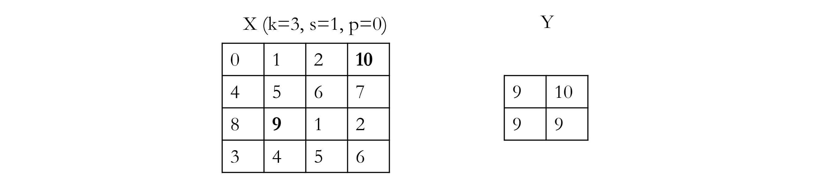
2D Convolution

Convolution is an affine transformation.
Each receptive field generates aone output value: sparse connection
# kernels = # output feature maps
Output size: $(c_0,o_h,o_w)=(c_o,\lfloor\frac{n_h+p_h-k_h}{s_h}\rfloor+1,\lfloor\frac{n_w+p_w-k_w}{s_w}\rfloor+1)$

Share the same parameters across different locations: reduce parameter, location invariant,

Implementation: Receptive fields across feature maps are concatenated into to one column.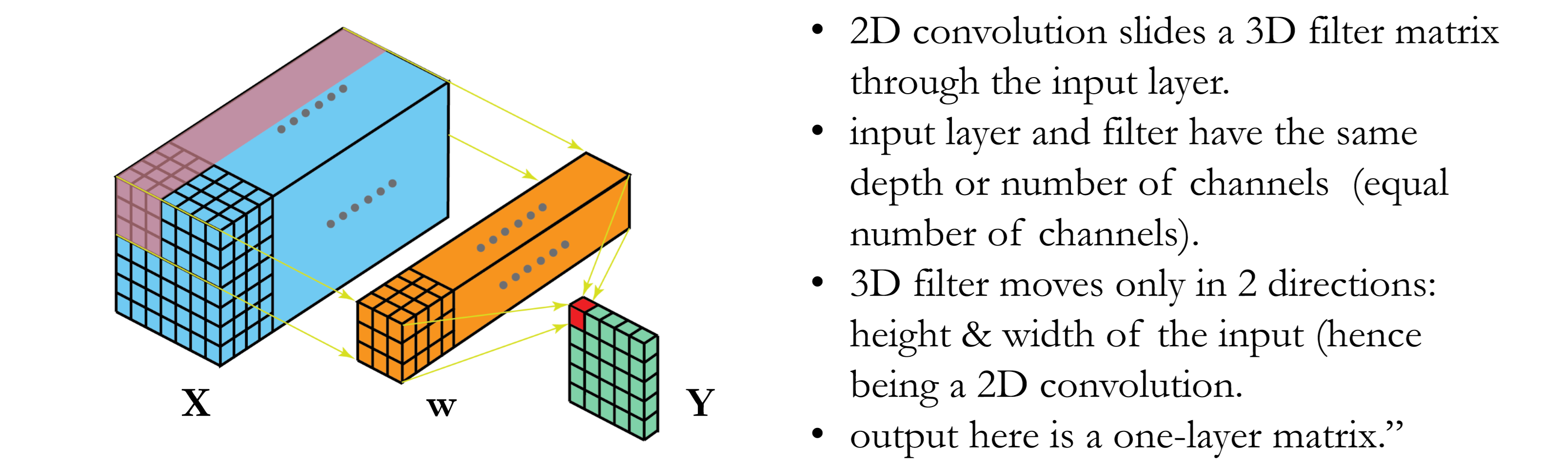

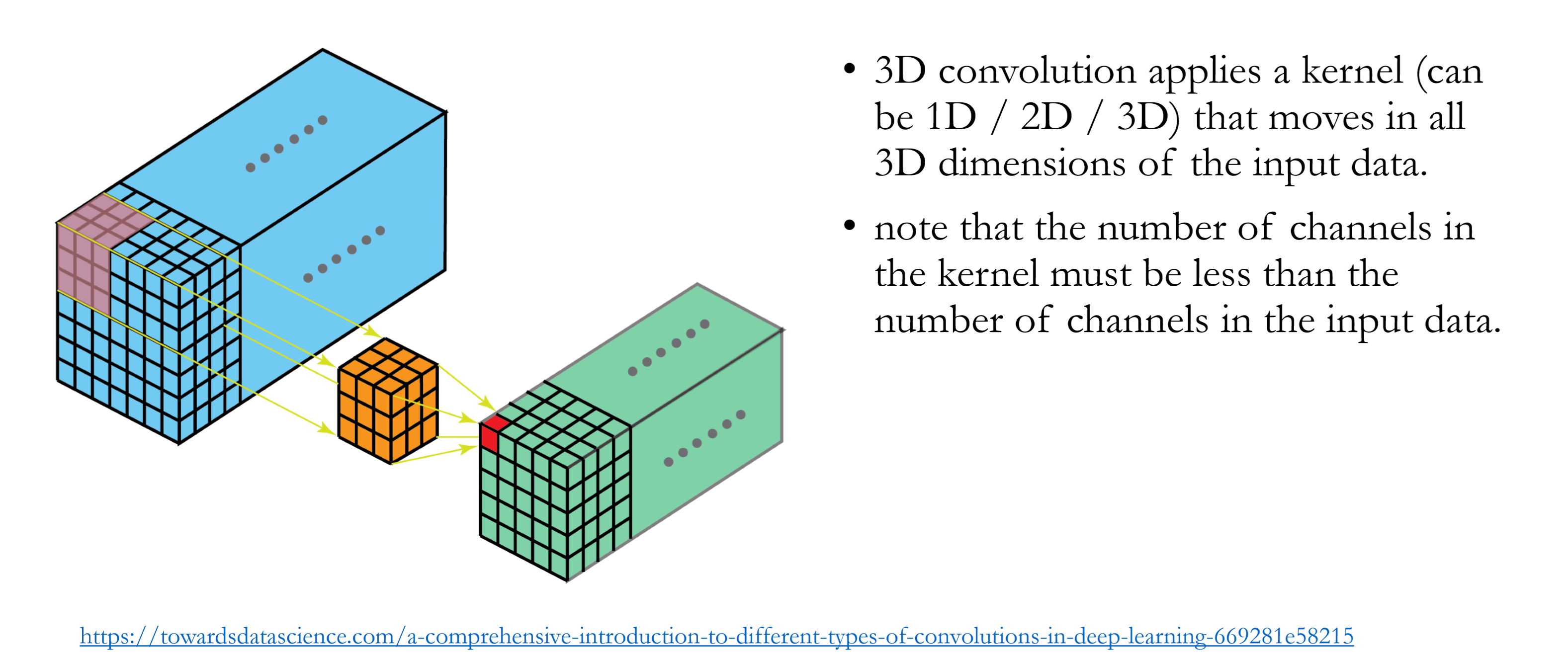
3D Convolution

Average & max pooling

• Aggregate the information from each receptive field.
• The output is invariant to some variations of the input. eg. rotation.
• Stride is usually > 1 to reduce dimensionality
• Pooling is applied to each channel / feature map separately

• Information will be lost from pooling but local “useful” information remains.
• We don’t need to keep as many features as possible because we want to derive higher levels of abstraction. e.g. from simple edges to parts of objects

ConvNet Architecture

Neocognitron

• Hierarchical Feature Extraction + Multi-Layer + Hand-crafted weights.

LeNet 1-5

• Small CNN with convolution + pooling (subsampling)

AlexNet

• GPUs (instead of CPUS): Fast training
• Ensemble modelling
• ReLU: Reduce the chance of gradient vanishing
• Dropout: Multiple the outputs (h) with scale 1/(1-p); Regularization (Similar to L2 norm)
• Image augmentation: Done on-the-fly during training, so no need to store entire (augmented) dataset and occupy memory. Random operation for training; No random operations during test, Make predictions by aggregating the results from all augmented images.(Voting)

VGG

• Uniform kernel size
• Consecutive convolution layers

InceptionNetV1

• Parallel paths: inception block (1x1 convolution), insert the 1x1 convolution layer with a small number of kernels to fuse the channels from the input tensor and reduce the computational cost for the next convolution
• Complexity optimization
• Average pooling: Reduce model size (less overfitting); Reduce time complexity
• New image augmentation methods

InceptionNetV2

• Batch Normalization
  Computes the mean and variance over mini-batch samples’s features.
  Normalize every neuron of each sample.
  Applied after linear transformations and before activation.
  (z = relu(BN(conv/ fc(x))) or z = BN(relu(conv/ fc)))
  Accumulates the mean and variance from every batch during training, and then apply them during test

InceptionNetV3

• Spatially separable convolutions(Factorization of the kernel): Reduce computation cost $\to$ train faster ( 7x7 == 1x7 and 7x1 (receptive field))
• Label smoothing: prevents network from becoming over-confident and optimizing towards values that cannot be achieved

ResNet

• Skip/Residual-connection: Reduct gradient vanishing.

XceptionNet

• Depth-wise spatial convolution: 2D Convolution applied to each channel independently; Number of input channels = number of kernels = number of output channels: $c_i=c_o$, Each kernel has a single channel
• Pointwise convolution: Normal 2D convolution with kernel height and width: 1x1

Neural Architecture Search (NAS)

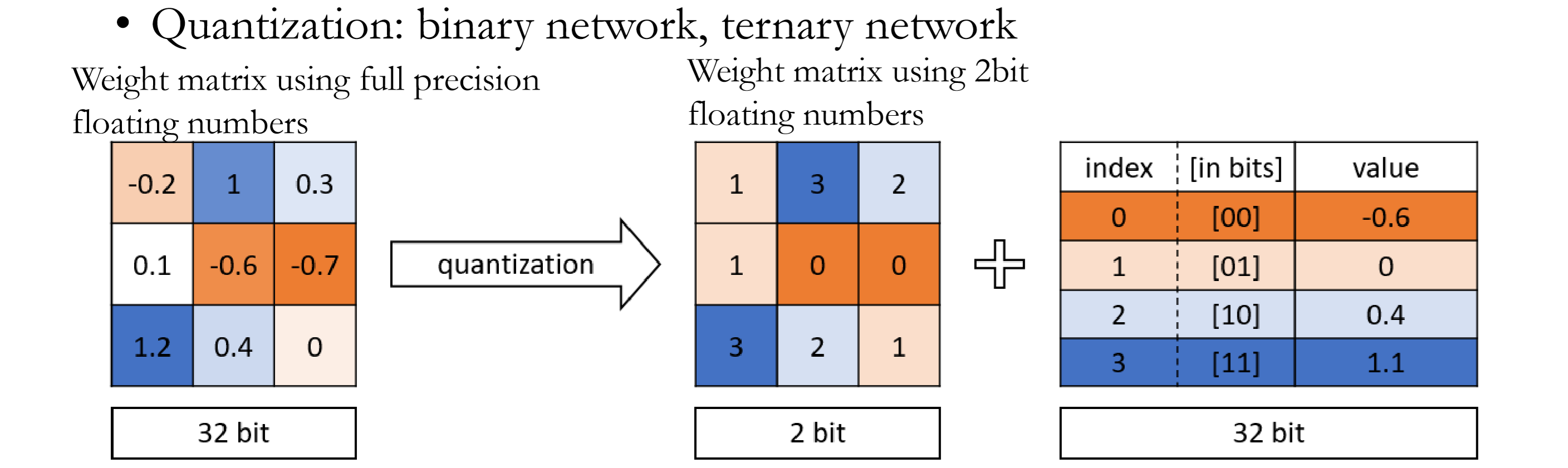
• Model Compression: Prune layers, Low-precision representation
  

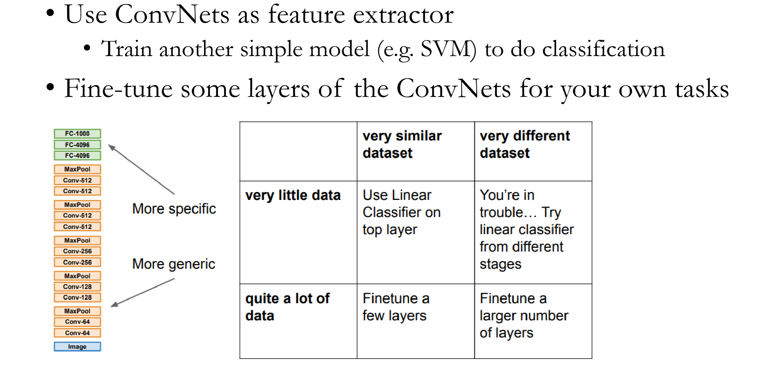
Transfer Learning with DCNN

1. Train model (or use someone else’s model) on ImageNet 2012 training set
2. Re-train classifier on new dataset //Just the top layer (softmax or SVM)
3. Classify test set of new dataset