Paper: https://www.arxiv-vanity.com/papers/1712.01208/
Introduction
There exists various data access patterns, and correspondingly various choices of index structure.
B-tree: range request (from sorted array)
HashMap: single key look-ups (from unsorted array)
Bloom filters: check for record existence
If data is from 1 to 1000, we don’t actually need a tree structure, we just need to use a direct look-up for the key. This example shows that One size does not fit all.
Traditional data structures make no assumptions about data, they only rely on the size of data.
While using ML, we try to learn the distribution of data, We use data complexity instead of data size to construct a suitable index. In this way, we can achieve huge performance improvement.
There are also many other data structures and algorithms in database system, we can apply the idea of using ML to change the design of them.
Basically, we want to use ML techniques to enhance traditional index structures or even replace them to get a better performance.
Range Index (B-tree)
Range Index Models are CDF Models
B-tree can be viewed as a model which takes the feature’s key as input and predict the position of the feature. Usually a B-tree maps a key to a page, and then searches within this page. Which means B-tree outputs a position, and searches within $[pos, pos+page_ size]$. i.e., by normal B-trees, the error is defined by the pagesize.
model:f(key)->pos, searches from $[pos-err_{min},pos+err_{max}]$
we can search in this range to find the exact right record.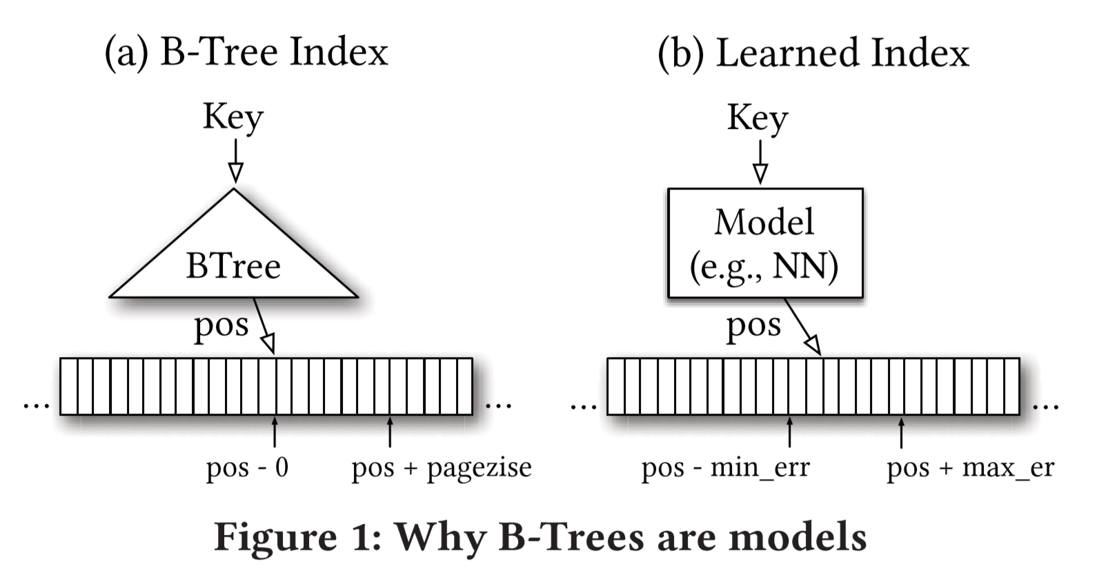
We don’t care about generalization, we only care about the data we have.
So B-tree is actually building a model of Cumulative Distribution Function:
$p=P(x\leq key)*nums_of_Keys$
p is the predict position from key.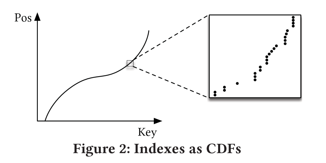
For example, if your data is a Gaussian Distribution, most of your data is around the middle, and the learned index can allocate more trees in that area because of this information.
Potantial Advantages of learned b-tree models:
smaller index: less main-memory storage
faster lookup
more parallelism: sequential if-statement is exchanged for multiplications
assume read-only
A First Naive Learned Index
200 M records of timestamps (sorted)
two-layer fully-connected neural network
32 neurons per layer
ReLu activation functions
train this model to predict the position of the timestamp
measure the look-up time for a randomly selected key (averaged over several runs)
look-up with B-tree: 300ns
look-up with binary search: 900ns
look-up with Model: 80000ns (1250 predictions per second)
This model is a naive version and doesn’t work well and we find this model is limited in the following ways:
- Tensorflow is designed for large models, not small models like this.
- B-tree can easily overfit the training data and can predict the position precisely. For database system, overfitting is not that bad, you get a database, you know the data you’re trying to search, and there are no other data outside to generalize,
While learned index can easily narrow the space from 100M to 10k but have trouble in narrowing the space from 100M to hundreds, which is “the last mile of learned index”, in other words, learned index has problems being accurate at the individual data instance level. - B-trees are cache efficient, they keep the top nodes always in cache and they access other pages if needed. In contrast NN need to load the all parameters into memory to compute a prediction and have a high cost in the number of multiplications.
- For classic machine learning problems, the ultimate goal is the desired average average error, but we look for the index, hoping to get the best prediction, and finally hoping to find the true position of the key. Search does not make advantage of this prediction, the question is what is the right search style given an approximate answer
RM-Index (B-tree)
The Learning Index Framework (LIF)
LIF is an index optimization system. Given a set of index data, LIF automatically generates multiple sets of hyperparameters, and automatically optimizes and tests to find the optimal set of configurations.
When applied in a real database, LIF will generate an efficient index structure based on C++. LIF focuses on small models, so many unnecessary costs for managing large models must be reduced(Use a specific model structure to reduce runtime overhead, such as pruning, removing redundant if-else, direct memory access, etc.), now we can optimize the model prediction to within 30ns.
LIF is still an experimental framework and is instumentalized to quickly evaluate different index configurations.
Recursive Model Index
The real data distribution function is often between the two: in general, it satisfies a change trend, but the part is a piecewise function (the piecewise function of daily data may be different)
In that case we use the idea of Mixture-of-Experts and propose Recursive Model Index to solve the problem of “the last mile of learned index”
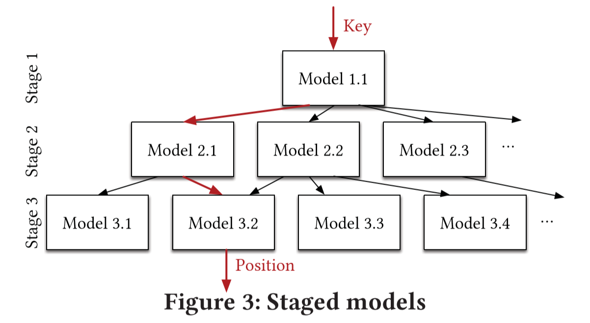
We use a hierarchical experts, i.e. a hierarchy of models.
At each stage, take the key as input and based on it to pick another model, until final stage predicts the position.
Every model is like an expert for a certain range and may has a better prediction.
- Such a multi-layer model structure is not a search tree, and multiple stage 2 models may point to the same stage 3 model. In addition, at the lowest level, in order to ensure that the smallest and largest deviations can be controlled, we can also use B-Tree to complete the final index.
- Each model does not need to cover the same amount of records like B-trees do.
- predictions between stages don’t need to be the estimate of position, but can be considered as picking an expert which has a better knowledge about certain keys.
RMI has several benefits:
- It separates model size and complexity from execution cost
- It is easy to learn the overall data distribution
- Divide the entire space into smaller subranges. Each subranges is similar to a B-tree or decision tree, making it easier to solve the last-mile accuracy problem.
- No search process is required in-between stages. For example, the output y of model 1.1 is an offset, which can be directly used to select the model of the next stage.
Hybrid Indexes
Another advantage of the recursive model index is that we are able to build mixtures of models.
top-layer: a small ReLU neural net —- they can learn a wide range of complex data
bottom: simple models like linear regression(inexpensive in space and execution), or B-trees if the data is particularly hard to learn(worst case)
Such a recursive model has several advantages:
- It can learn the shape of the output data well.
- Through stratification, you can basically use B-Tree or decision tree to obtain very high search efficiency.
- Different stages can use penetration to initialize the model instead of searching, which makes it easier to refactor and optimize the programming language.
Search Strategy
- Model Biased Search:the default search strategy, based on binary search, the new intermediate point is based on the standard deviation $\sigma$ of the last layer of model settings
- Biased Quaternary Search:search three points at the same time, $pos-\sigma, pos, pos+\sigma$ . Requires CPU to obtain multiple data addresses in parallel from main memory
- how to deal with large address spaces
- how do we deal with not able to assume that the end location is ordered
if pages are in disks or other seperate devices they may not be in order
it’s an engineering issue
Indexing Strings
Training
Results
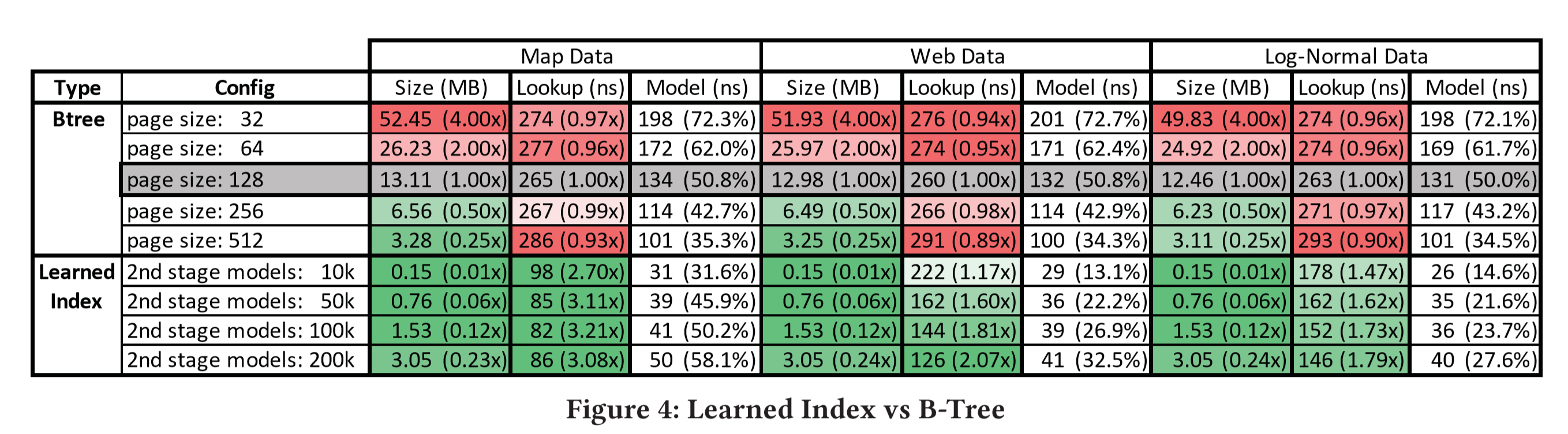
trade-off between memory and latency
Map data: relatively linear
Web data: (timestamp) complex, a worst case
Log Normal Data: non-linear integers, heavy tail
2nd stage: linear models have the best performance.
For the last mile we don’t need to execute complex models.
- Histogram: B-Trees approximate the CDF of the underlying data distribution. When we use histograms as a CDF,this histogram must be a low error approximation of the CDF. However, this requires a large number of buckets, which makes it expensive to search the histogram itself. And almost every bucket has data insides, only few buckets are empty or too full. The solution to this case is B-Trees, so we’ll not discuss Histogram individually.
- Lookup-Table: Lookup-table is another simple alternative to B-trees. A lookup table is an array that replaces runtime computation with a simpler array indexing operation(Wikipedia).
Performance comparison: linear search vs binary search.
https://dirtyhandscoding.wordpress.com/2017/08/25/performance-comparison-linear-search-vs-binary-search/ - FAST: a highly SIMD optimized data structure, allocate memory in the power of 2, leading to significantly larger indexes
- Fixed-size B-Tree & interpolation search
- Learned indexes without overhead: a multivariate linear regression model at the top and simple linear models at bottom
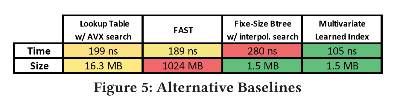
Because the binary search of string will be more time-consuming, the search strategy proposed above(learned QS with quaternary search) can improve efficiency more significantly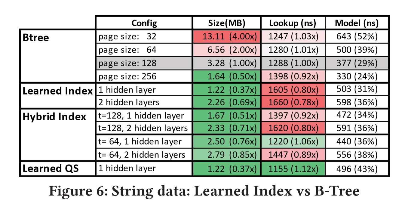
Point Index (hash)
Point Index, as the name suggests, is to search for the position corresponding to the key, which is Hashmap. Hashmap is naturally a model, the input is the key and the output is the position. For Hashmap, in order to reduce conflicts, it is often necessary to use a much larger number of slots than the number of keys (the paper mentions that a hashmap usually has 78% extra slots in Google). For conflicts, although there are linked-list or secondary probing methods to deal with, their overhead is not small. Even using sparse-hashmap to optimize memory usage, the performance is 3-7 times slower than hashmap.
Therefore, the learned model can reduce the additional memory overhead on the one hand, and reduce the overhead of some conflicts on the other hand (Hashmap can avoid conflicts by using more slots. If there are few conflicts, it will be difficult to optimize the index Time Because Hashmap is inherently constant complexity, the goal here is to reduce the memory overhead of Hashmap while ensuring indexing time). As shown in the figure below, the Learned Hashmap can not only reduce conflicts, but also make better use of memory space under the same number of slots.
The point index does not need to ensure that the records are continuous (maxerr and minerr do not need to be considered), so the trained model F fit CDF is easier to meet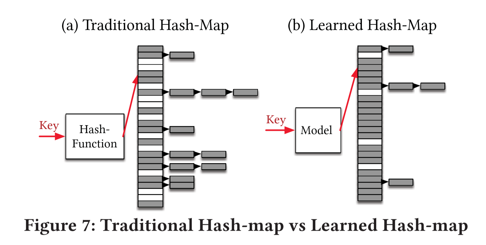
After the hash function is replaced with the model, the index time is not shortened, but the key space is indeed effectively reduced, which improves the space utilization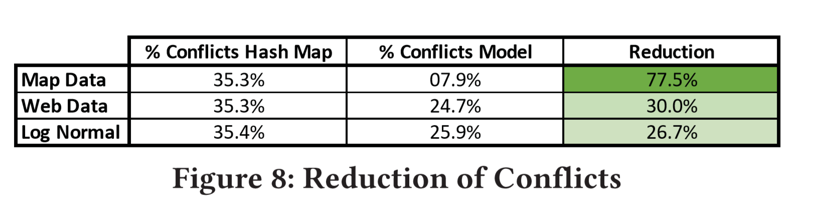
Existence Index (Bloom-Filters)
Although Bloom filters allow false positives,
for many applications the space savings outweigh this drawback
Considering the usage scenario of the existence index is usually to first determine whether the record exists in the cold storage, and then access the data through disk or network. So the latency can be relatively high, so that we can use more complex RNN or CNN models as classifiers.
Related Work
B-Tree and Variants
Over the last few years, a variety of different index structures have been proposed, such as B+-trees, red-black trees, all aiming at improving the performance of original main-memory trees. However, none of the structures have learned from the data distribution.
While using our hybrid model, we can combine the existing index structures with the learned index for further performance gains.
Perfect hashing
Perfect hashing tried to avoid conflicts without learning techniques.
The size of perfect hash function relies on data size.
In contrast, Learned hash function can be indenpendent of data size.
What’s more, perfect hash is not suitable for B-trees and Bloom filters.
Bloom filters
Our existence indexes directly make use of the current bloom filters by adding a ML model before the simple bloom filter and creating a classification model.
And in addition we can also use our learning model as a special hash function to seperate the keys and non-keys.
Modeling CDFs
Our models for both range and point indexes are closely tied to models of CDF.
How to mostly model CDF remanins an open question.
Mixture of Experts
Our RMI architecture builds experts for subsets of the data and in this way we can make our model size indepentent on model computation.
So we can create models that are complex but still cheap to execute.
Conclusion and future work
Other ML Models
We combine some simple neural networks with the existing data structures, and there are definitely more ways to do the combination which are worth exploring.
Multi-Dimensional Indexes
Models like NN are extremely good at handling multi-dimensional data, and the learned model could be used to estimate the position given various attributes.
Learned Algorithms beyond indexing
Learned Algorithms can also be applied to other data structures and CDF models are beneficial to join and sorting operations as well.
GPU/TPU
All we have been doing is to learn data pattern and use it in data structure design.
We are now having TPU/GPU which are vector processors and vector multiplies become very cheap.
We can make use of this property and construct new data structure along with ML techniques to speed up the look-up time and get better performance.
In summary, we have demonstrated that machine learned models have the potential to provide significant benefits over state-of-the-art indexes, and we believe this is a fruitful direction for future research.
B-tree indexes and CPU caches
https://www.researchgate.net/search.Search.html?type=publication&query=%20B-tree%20indexes%20and%20CPU%20caches
Making B+-Trees Cache Conscious in Main Memory
http://www.cse.iitb.ac.in/infolab/Data/Courses/CS632/2006/Papers/cache-b-tree.pdf
Adaptive Range Filters for Cold Data: Avoiding Trips to Siberia
http://www.vldb.org/pvldb/vol6/p1714-kossmann.pdf
Cuckoo Filter: Practically Better Than Bloom
https://www.cs.cmu.edu/~dga/papers/cuckoo-conext2014.pdf