Convolution

Convolution is a linear transformation and the output is the feature of the input.

1D: text processing
2D: image processing
3D: 3D data, CT, microscopy, etc

mD: m dimensions where the kernel is shifted

1D convulution

$\boldsymbol{y}_t=\sum_{i=0}^{k-1}\boldsymbol{w}_i\times \boldsymbol{x}_{t+i}$

This operation is actually cross-correlation, but we call it convolution.
$\boldsymbol{w}$: kernel/filter, length: k
$\boldsymbol{x}$: input, length: n
$\boldsymbol{y_t}$: the output feature, length: o
The area of input data where a kernel applied is called the receptive field, each receptive field is corresponding to a single output feature $\boldsymbol{y_t}$, which means, every time the kernel is shifted, there’s a new output $\boldsymbol{y_t}$.

Every cell of vector $\boldsymbol{w}$ is a parameter to be learned. In the 1D convolution below, Every output is generated from 3 input data x and these 3 cells is called a receptive field. We move the kernel along the input data until we cannot move further.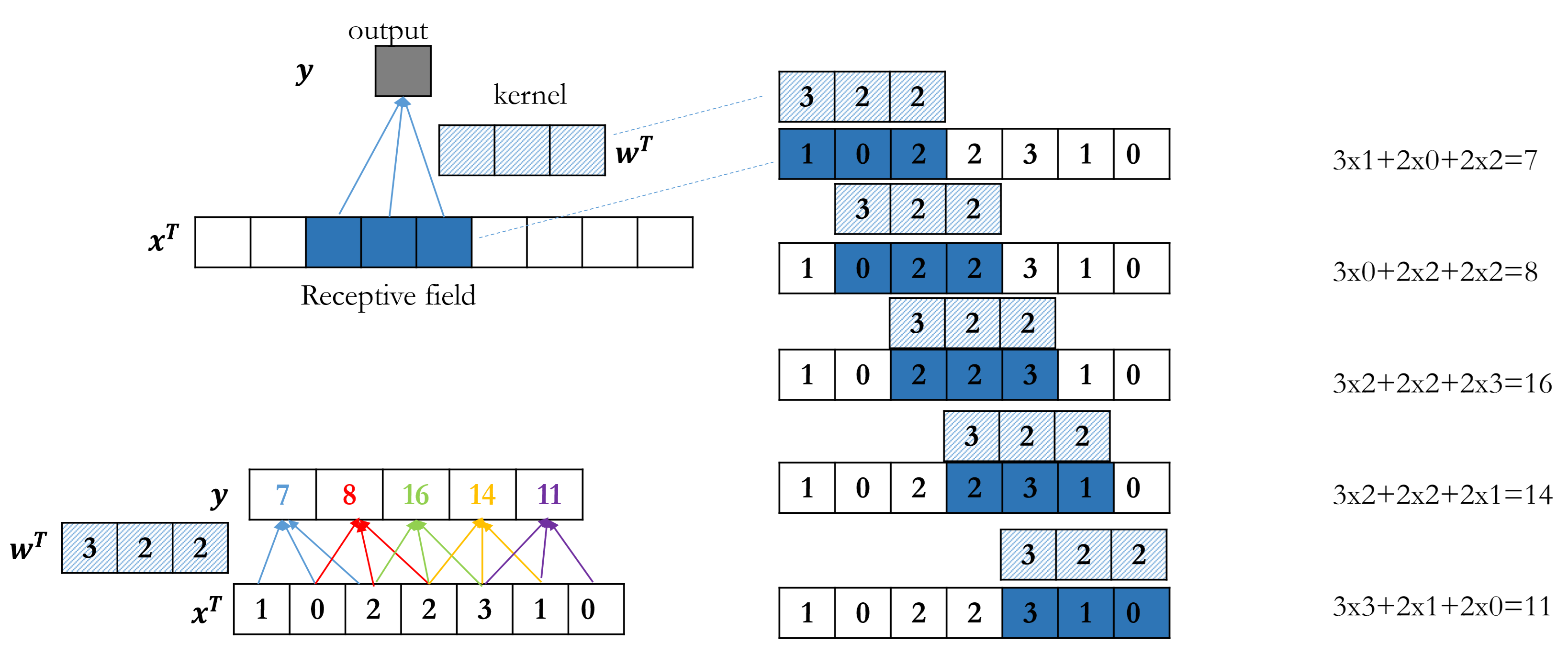

Benefits of Convolution

Sparse connections
Each output is only connected to the receptive field instead of the whole input data(fully-connected) $\to$ fewer parameter and less overfitting
Weight sharing
Regularization
Less overfitting
Location invariant
Make the same prediction no matter where the object is in the image. (the same values of receptive field lead to the same output regradless of the place of the receptive field)

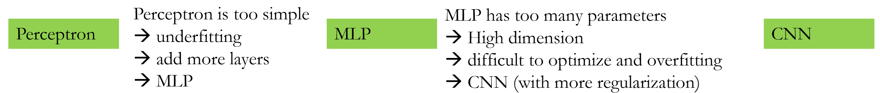
Perceptron, MLP and Convolution

MLP

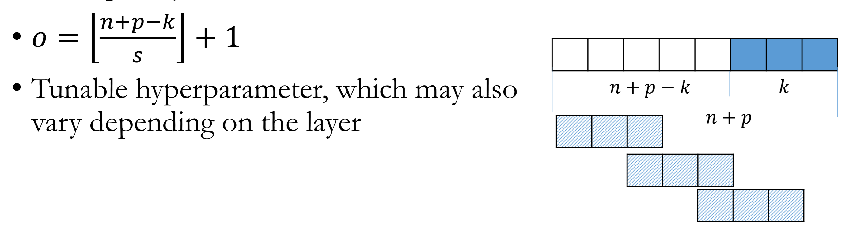
Padding

When stride = 1:

$o=(n+p)-k+1$

$o$ : output length $\quad n$ : input length $\quad k$ : kernel length $\quad p$ : padding length
$p = 0\to$ valid padding $\qquad p=k-1\to$ same padding ( left: $p/2$, right: $p/2$ ).
$p$ can be set manually or automatically.
Pad with 0 for convenience.

Stride

Stride: how many steps to move towards the next receptive field.
Larger stride sizes skip more elements, effective receptive field size increases quickly, one output contains larger range of information of deeper lever.
Meanwhile increasing the stride is computationally faster, since we compute less convolution.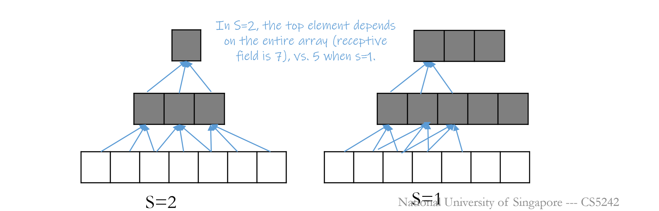
stride

$o=\lfloor\frac{n+p-k}{s}\rfloor+1$ $\to \frac{n+p-k}{s}\geq o-1$ $\to p\geq s(o-1)+k-n$ $\to p = max(0, s(o-1)+k-n)$

When stride > 1, output length cannot be equal to the input length.
“same” is defined as:

$o=\lceil \frac{n}{s}\rceil$

stride

Conv1D: forward & backward

Convert each receptive field to a column.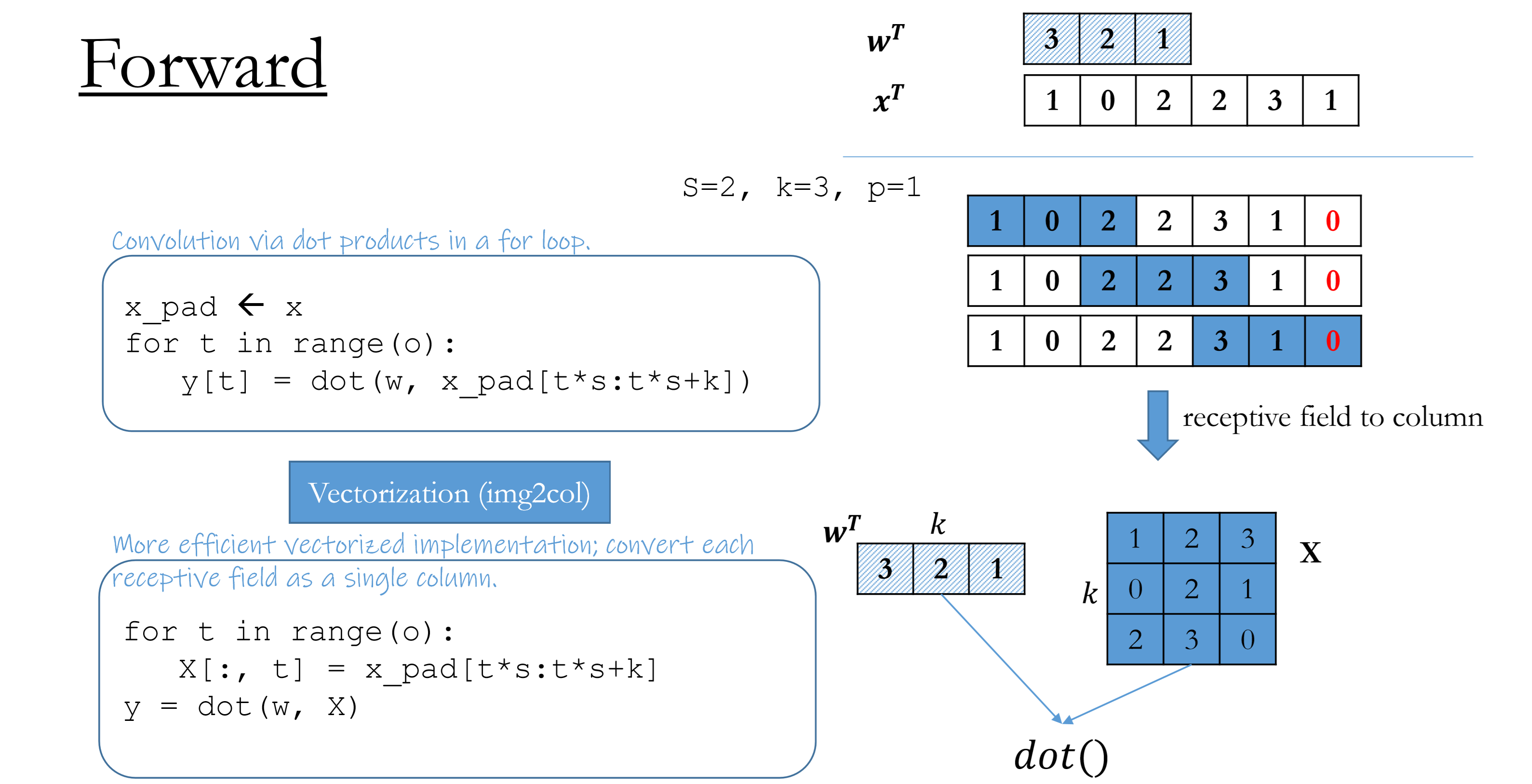
forward
backward

2D Convolution

Kernels move from left to right, from top to the bottom. (2 directions)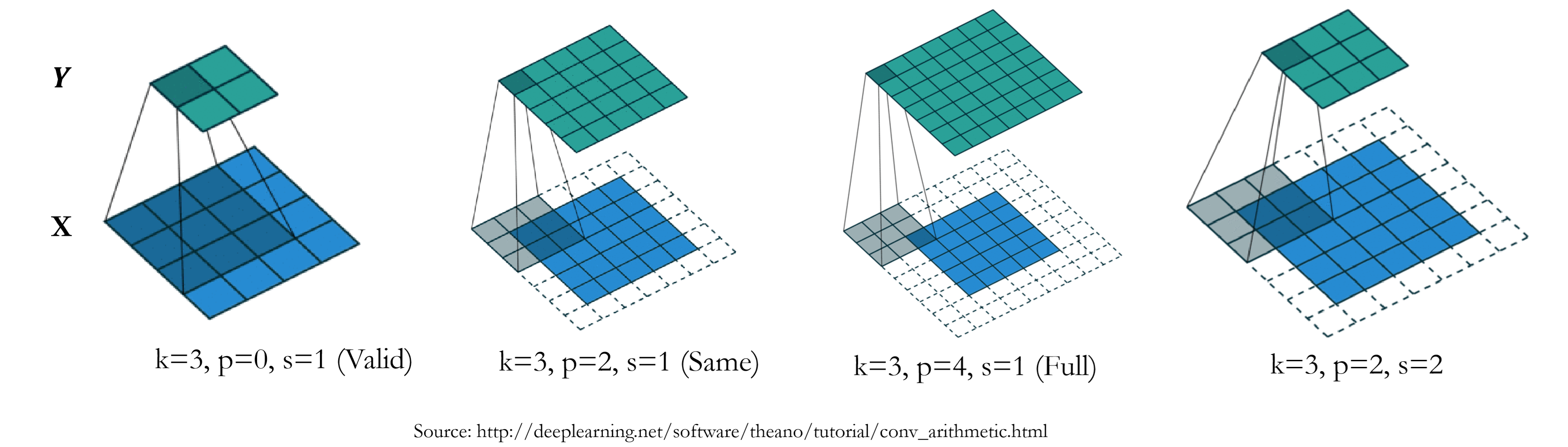

Single channel, single kernel

Convert each receptive field to a column.
Input $\mathbf{X}$ : $(n_h, n_w)$
Kernel $\mathbf{W}$ : $(k_h, k_w)$
Output $\mathbf{Y}$ : $(o_h, o_w)= (\lfloor\frac{n_h+p_h-k_h}{s_h}\rfloor+1,\lfloor\frac{n_w+p_w-k_w}{s_w}\rfloor+1)$
Computation cost: $O(k_h\times k_w\times o_h\times o_w)$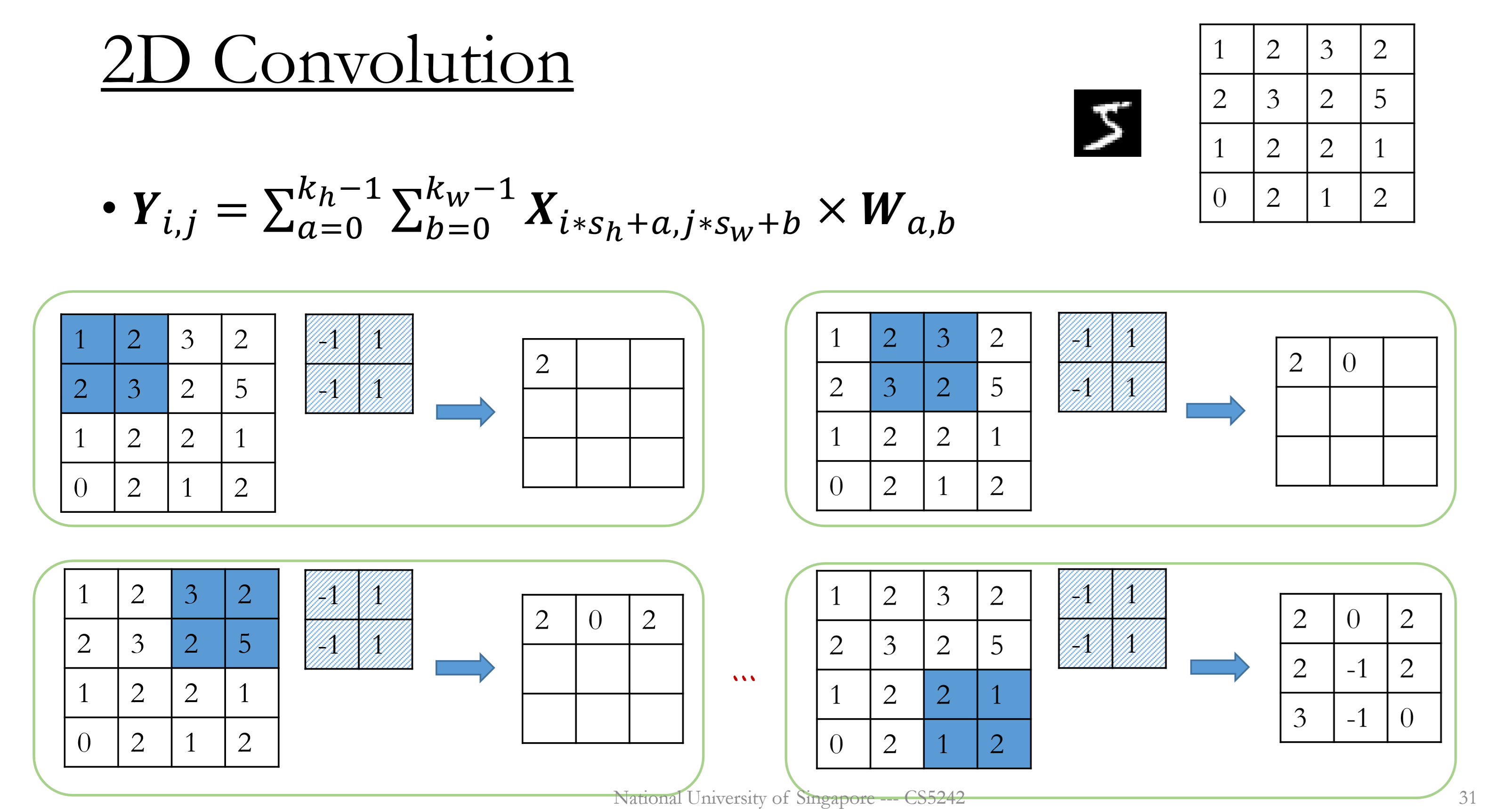
2d_single_kernel

Single channel, multiple( $c_o$ ) kernels

Applying multiple kernels (filters) $c_o$, all of the same stride and padding.
Convert each receptive field and each kernel to a column.
Parameter size: $c_o\times k_h\times k_w$
Output shape: $(c_0,o_h,o_w)=(c_o,\lfloor\frac{n_h+p_h-k_h}{s_h}\rfloor+1,\lfloor\frac{n_w+p_w-k_w}{s_w}\rfloor+1)$
Computation cost: $O((c_o\times k_h\times k_w)\times (o_h\times o_w))$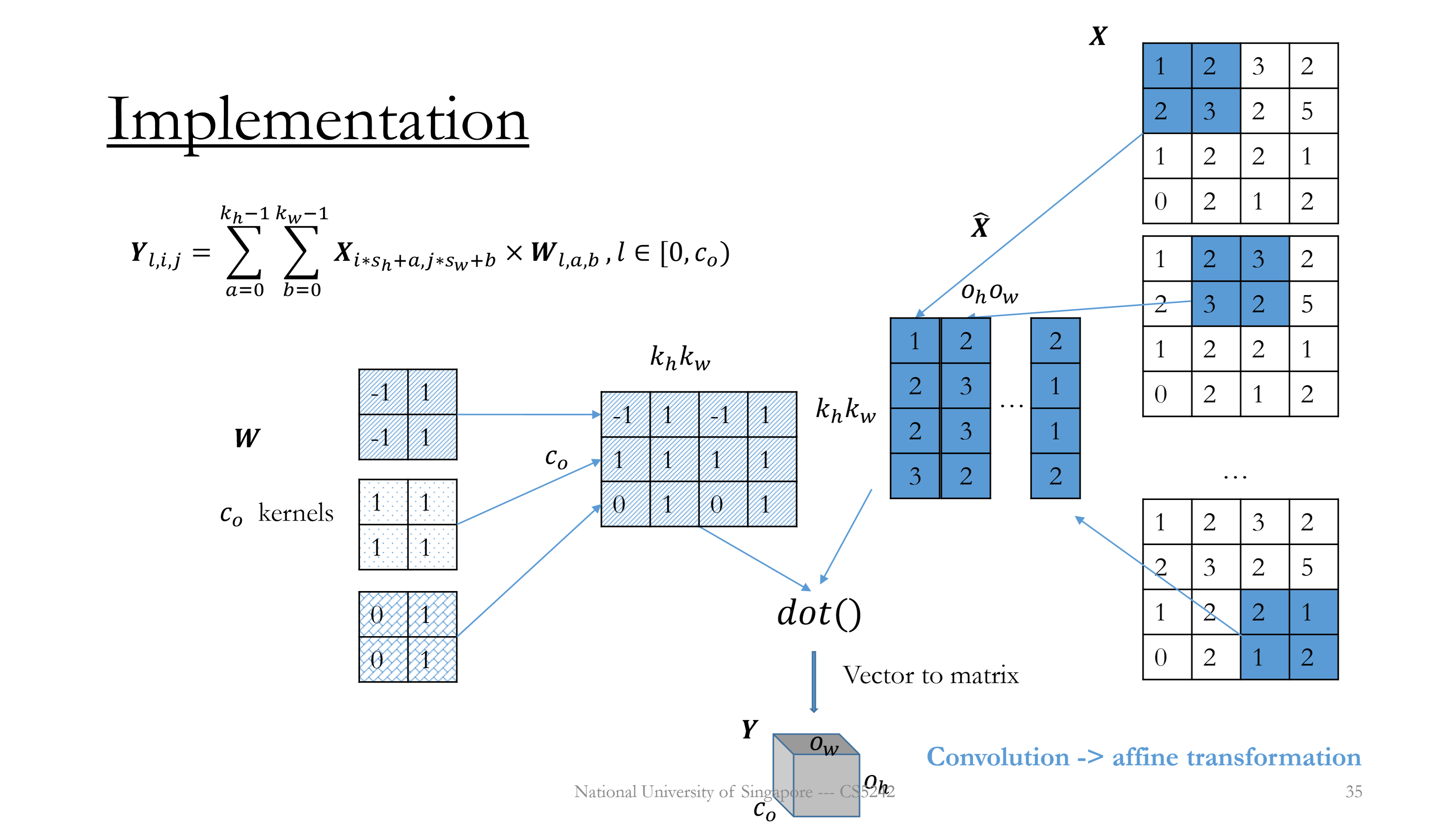
2d_s_m

Multiple( $c_i$ ) channels, multiple( $c_o$ ) kernels

Slide the window from left to right, top to bottom.
Receptive fields across feature maps are concatenated into to one column.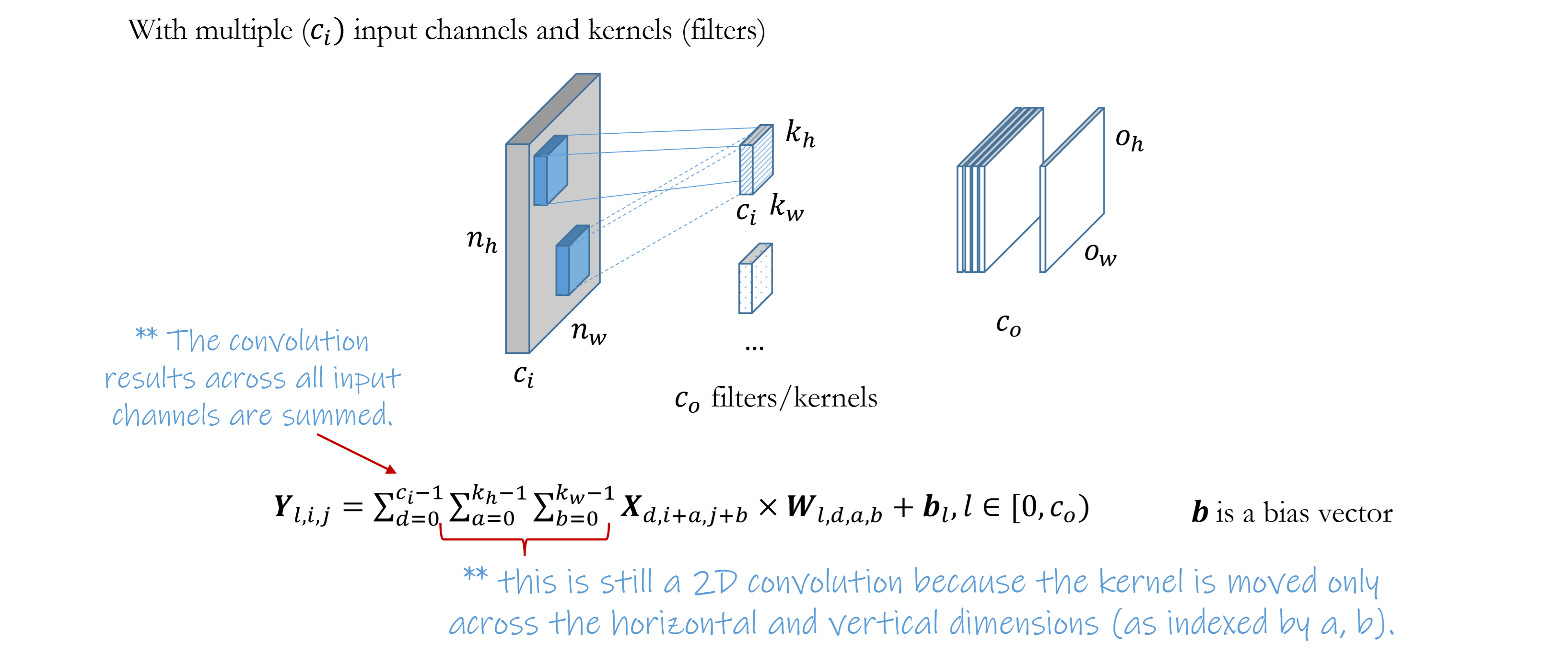
2d_m_m

Forward
Convert $\mathbf{X}$ into $\mathbf{\hat{X}}$ of size $(c_ik_hk_w\times o_ho_w)$
Reshape $\mathbf{W}$ into $(c_0\times c_ik_hk_w)$
$\mathbf{Y}=\mathbf{W\hat{X}}+\boldsymbol{b}$
Output shape: $(c_0,o_h,o_w)=(c_o,\lfloor\frac{n_h+p_h-k_h}{s_h}\rfloor+1,\lfloor\frac{n_w+p_w-k_w}{s_w}\rfloor+1)$
Computational cost: $O(c_o\times c_ik_hk_w\times o_h o_w)$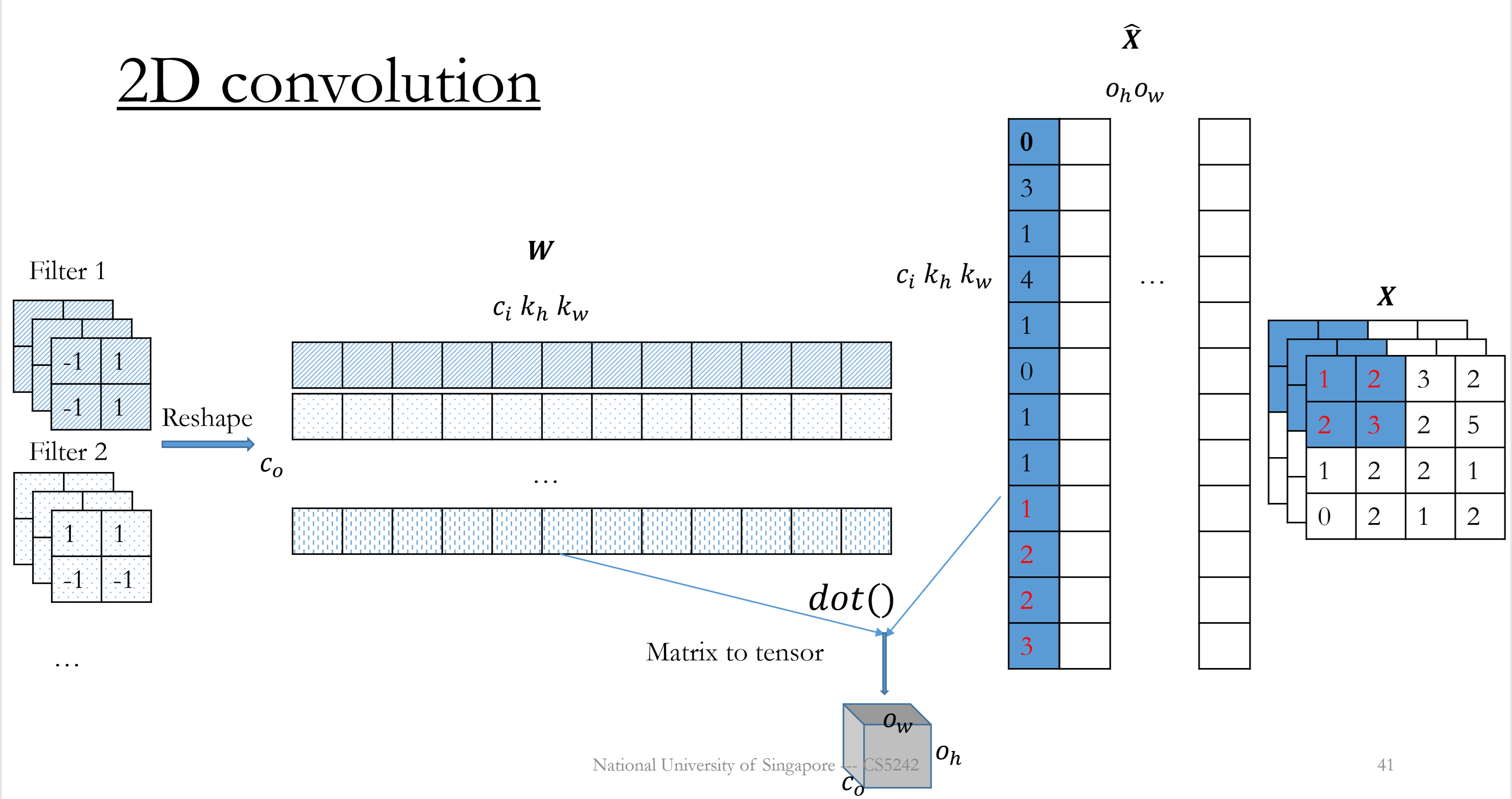
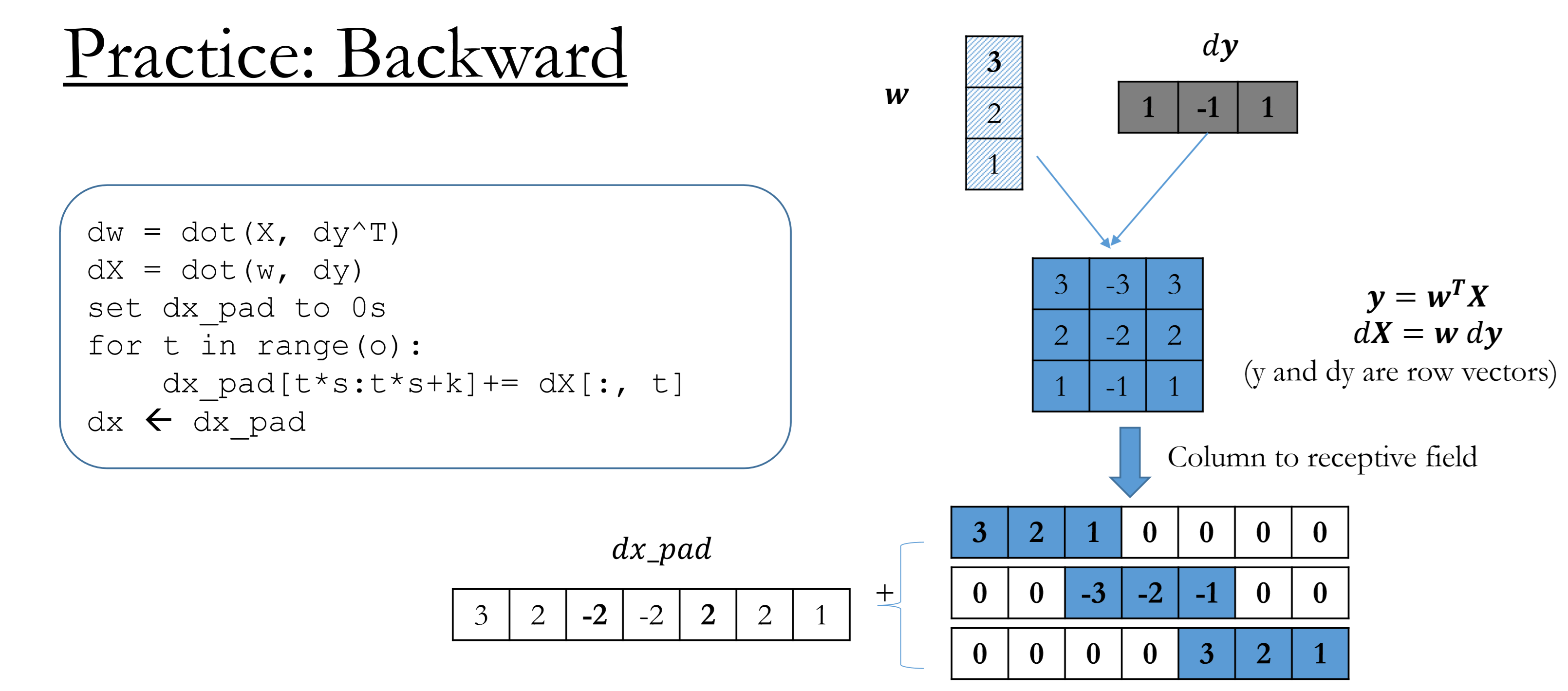
Backward
Given $\frac{\partial L}{\partial \mathbf{Y}}$
Compute $\frac{\partial L}{\partial \mathbf{W}}=\frac{\partial L}{\partial \mathbf{Y}}\mathbf{\hat{X}}^T\quad \frac{\partial L}{\partial \mathbf{\hat{X}}}=\mathbf{W}^T\frac{\partial L}{\partial \mathbf{Y}}$
Column to receptive field transformation to get gradient w.r.t original $\mathbf{X}$

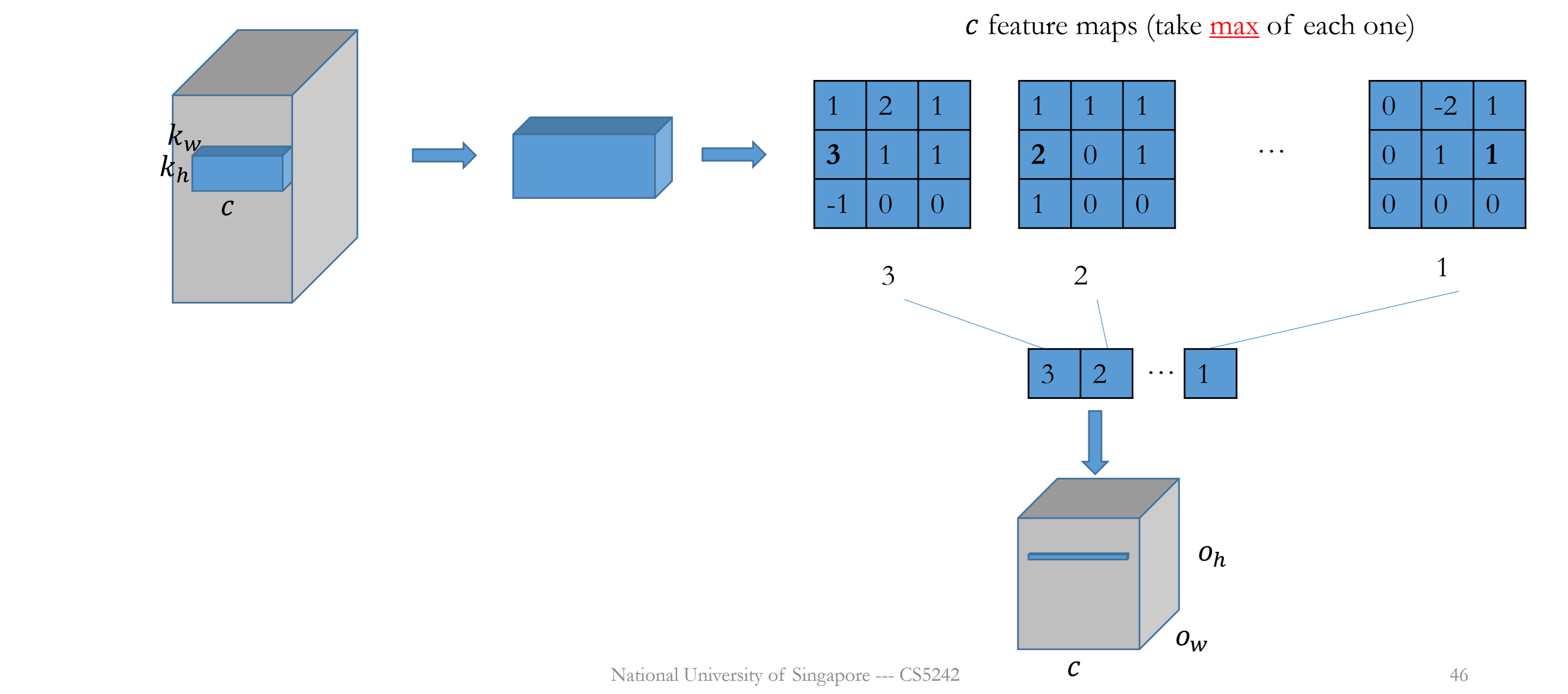
Pooling

No parameter, applied to each channel respectively.
Padding and stride can be applied.
# input channels = # output channels
i.e., $c_i=c_o=c$

Max pooling

max_p

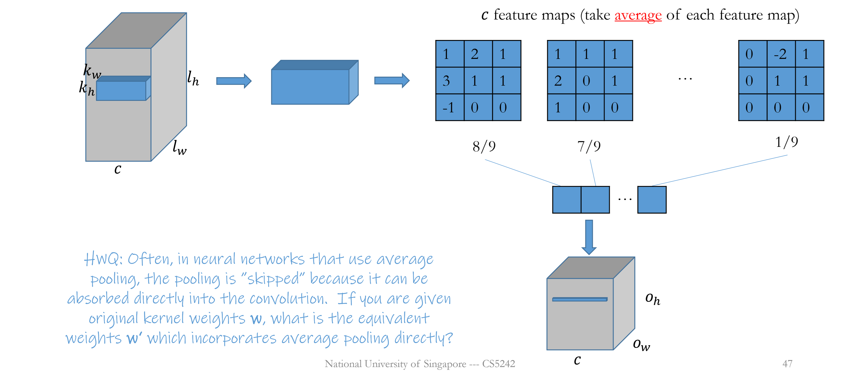
Average pooling

avg_p

Effect of pooling

Reduce the feature size and model size
Max pooling: invariant to rotation of the input image
Average pooling: is usually skipped, can be replaced by convolution (sum of weighted input); much cheaper(no weights)