Training Deep Networks

Stochastic Gradient Descent

Various GD’s problems and advantages

1. Forward computer the average loss among:
   • all training samples (GD)
   • randomly pick a single training sample (SGD)
   • randomly pick b training samples (mini-batch SGD)
2. Backword compute the gradient of each parameter
3. Update every parameter according to its gradient

Problems of GD:

• local optimum: stop updating when every parameter is at its local optimum. (This is a rare case)
• saddle point: we may not even arrive at a local optimum.
• Efficiency: has to load all data to compute the update, with high memory cost and high computation cost per iteration.

Advantage of SGD:

• more efficient in terms of memory cost and speed per iteration.
• avoid local optimum efficiently: although $\frac{\partial J^{(k)}}{\partial w}=0$ , $\frac{\partial J^{(i)}}{\partial w}$ (i != k) may not be zero.

Problems of SGD:

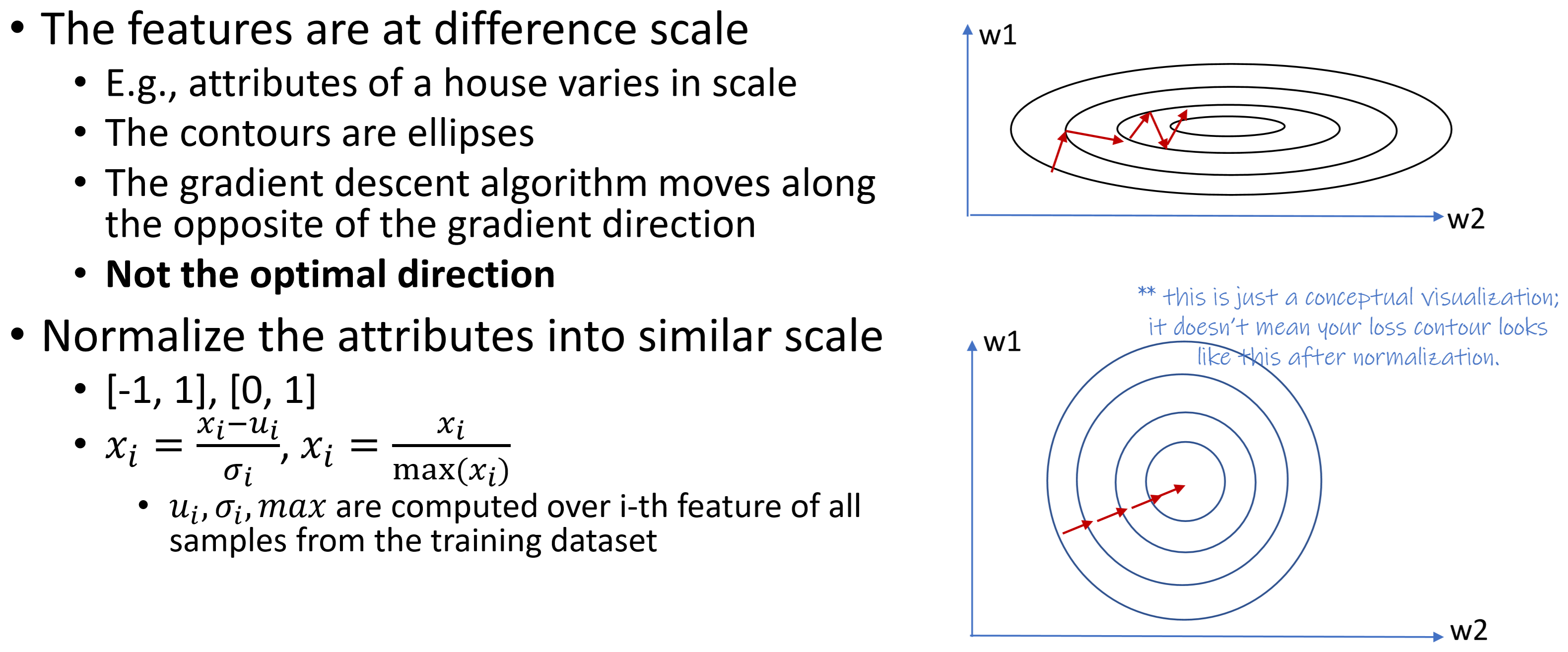
• not moving in the optimal direction for every step due to the stochastic process(minimizing loss for a single example but not for the whole training dataset and may not converge at all).

Advantages of mini-batch SGD:

• the derivation direction is more stable than SGD.
• Averaged on b samples, leading the faster convergence in terms of #iterations.

Efficiency compare:

• R for convergence rate: $R_{GD}>R_{mini-batch SGD}>R_{SGD}$
• T for time per iteration: $T_{GD}\leq T_{mini-batch SGD}\leq T_{SGD}$
• Tc for time to converage: $Tc=$#$\times T$ (number of iterations $\times$ time per iteration), it depends case by case. By experience, mini-batch SGD is the fastest to converge.

Batch Size

• larger batches are more accurate at estimating the gradient, better gradient does not equal to better performance due to the possibility of overfitting.
• GPU has limited memory, if all batch samples are processed in parallel, we should reduce batch size or use more GPU.
• Some hardware have better runtime with specific array sizes, e.g., for GPUs, powers of 2 are usually optimal.
• Training with small batch need small learning rate to reduce the noise and maintain stability due to the high variance in the estimated gradient, this trade-off may slow down the overall learning speed.
• Small batches act as regularizers with noisy approximated gradients.
• Using extreme small batches may cause the underutilization of multicore architectures and there is a fixed time cost below a certain batch size.

Loss Contour

Every point in the contour is a specific assignment of parameters, points on the same circle have the same loss value, points on the innermost circle have the minimum loss.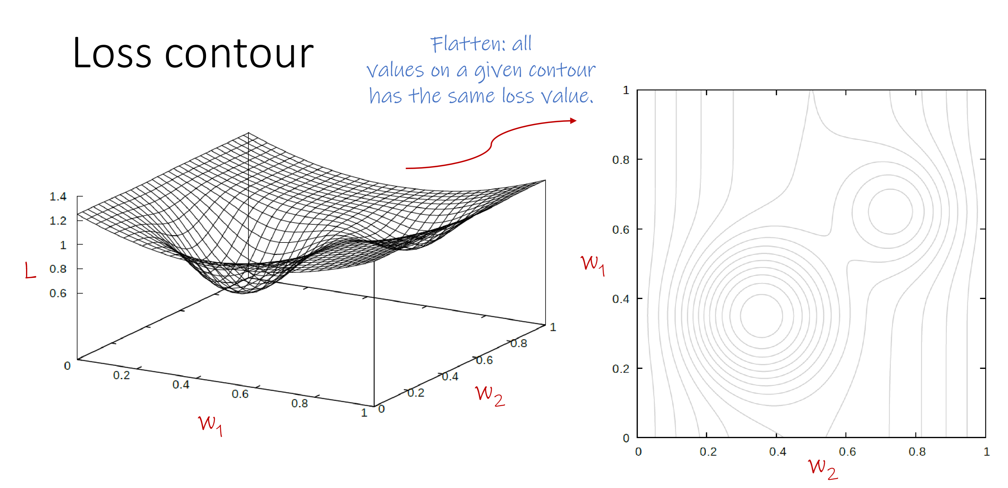

Evolution of mini-batch SGD

mini-batch SGD with momentum

Motivation：

• Gradients may dramatically change on a complex loss function.
• Hard to make progress on flat regions.
• Momentum smooths the gradients over past time, i.e., balance thes history and new gradient.

Algorithm:

$$v=\beta v+\alpha g$$ $$w=w-v$$

Adagrad

Motivation：

• Different dimensions have different gradients.
• We want a larger lr for small gradients and small lr for large gradients.
• Adagrad makes learning rates adapt to each dimension.

Algorithm:

$$s=s+g^2$$ $$w=w-\frac{\alpha}{\sqrt{s+\epsilon}}g$$

RMSprop

Motivation：

• Adagrad decays the learning rate that may lead slow progress at end.
• RMSprop guarantees that learning rate will not end up to 0 as time goes by.

Algorithm:

$$s=\beta s+(1-\beta)g^2\qquad moving\quad average$$ $$w=w-\frac{\alpha}{\sqrt{s+\epsilon}}g\qquad nomalize\quad the\quad gradient$$

Adam

Motivation：

• Conbine the momentum and adapted learning rate to smooth the gradients and adapt to various dimensions.

Algorithm:

$$v=\beta_1 v+(1-\beta_1)g\quad \hat v = \frac{v}{1-\beta_1^t}$$ $$s=\beta_2 s+(1-\beta_2)g^2\quad \hat s = \frac{s}{1-\beta_2^t}$$ $$w=w-\frac{\alpha}{\sqrt{s+\epsilon}} v=w-\frac{\alpha}{\sqrt{\hat s+\epsilon}}\hat v$$

Adam offers fast convergence.
Mainly for the first few iterations, when t gets large, the denominator goes to 1.

Convergence

Usually, convergence is considered w.r.t the optimized variable, i.e. weights of the network.

• For learning, however, because we’re not really interested in finding the optimum but having a good model that will generalize, we are interested in convergence of the loss.
• Convergence then refers to the loss plateauing.

Training tricks

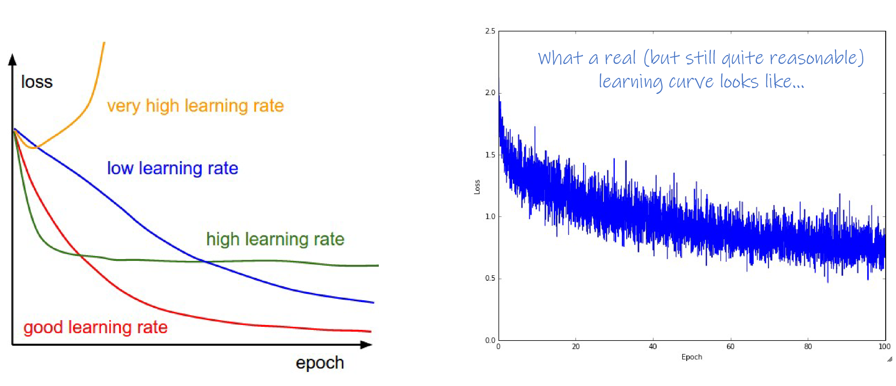
Learning Rate

Initialize lr with a large value and then decrease it gradually.
decay learning rate:

• step
• 1/t
• exponential $\alpha e^{-kt}$

Random parameter initialization

We want each unit to compute a different function and we do not want redundant parameters.
Random initializations can break symmetry.

• Gaussian, N(0, 0.01)
• Uniform, U(-0.05, 0.05)
• Glorot/Xavier : Gaussian N(0, sqrt(2/(fan_in+ fan_out))
• He/MSRA : Gaussian N(0, sqrt(2/fan_in))

General idea: keep variance of random values within some reasonable range. We want various parameters have the same scale/range.

• Too small variance: Z vanishing (Z = X W + b,)
• Too large variance: Z exploding

For bias vector: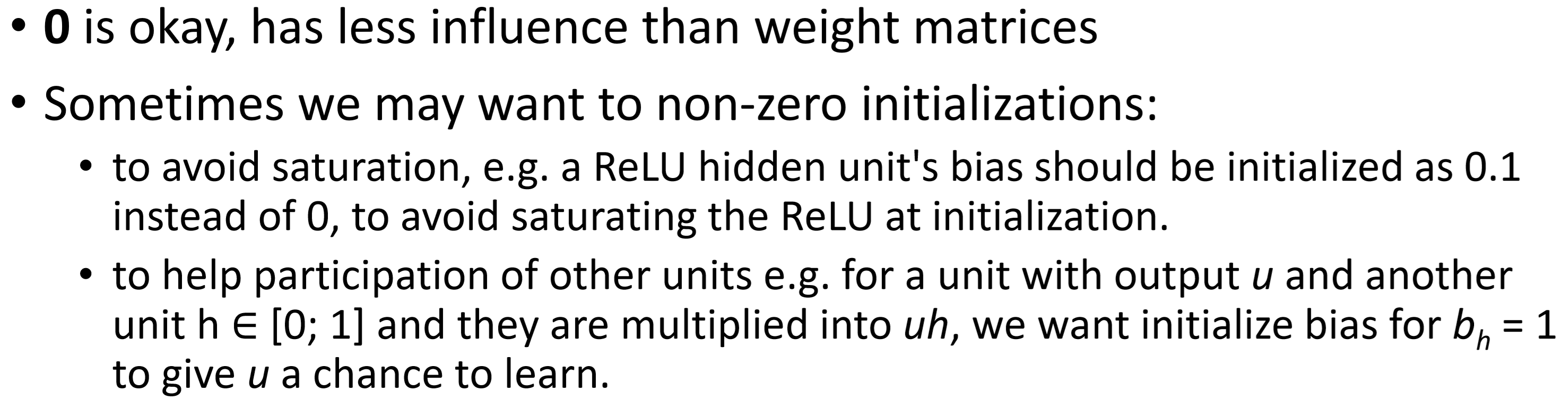

Data normalization

Overfitting and Underfitting

Underfitting

Low model capacity / complexity $\to$ model too simple to fit training data
High bias

• definition of bias (error): An algorithm’s tendency to consistently learn wrong things by not taking into account sufficient information found in the data

Overfitting

High capacity/complexity $\to$ fits well to seen data, i.e. training data
High variance
Cannot generalize well onto new data, so performs poorly on unseen data, i.e. test

• definition of Variance (errors): Amount that the estimates (in our case the parameters w) will change if we had different of training data (but still drawn from the same source).

A good model

Uses the “right” capacity / complexity to model the data and can generalize to unseen data.
Strikes a balance between under-and over-fitting, as well as bias and variance.
Because bias and variance derived from the same factor(model capacity), we cannot have both low bias AND low variance.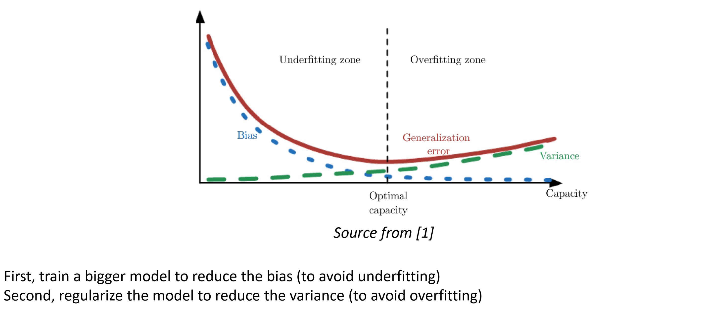

Regularization

Add L2 Norm

$\Phi$ is the flatten vector of all parameters:

$$J_{reg}=J+\frac{\lambda}{2}||\Phi||^2$$ $$\frac{\partial J_{reg}}{\partial w}=\frac{\partial J}{\partial w} + \lambda w$$

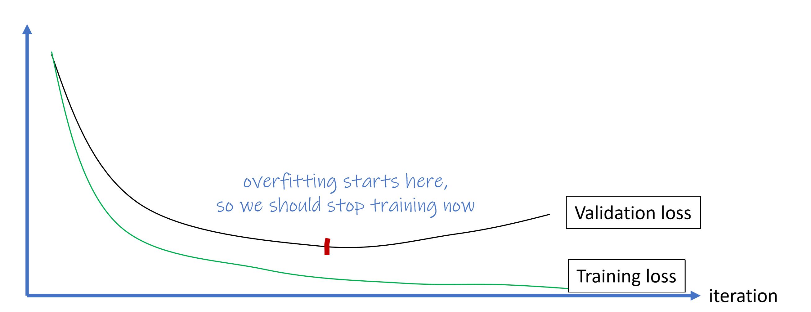
Stop early

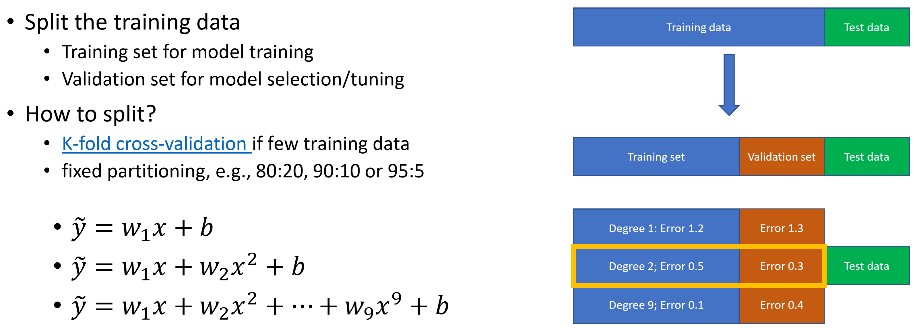
Model tuning and data splitting

Degree is a hyper-parameter or configuration knob.
Tuning the degree is called hyper-parameter tuning or model selection.
For complex models, there could be many such hyper-parameters, e.g. Learning rate of the gradient descent algorithm $\alpha$, Number of layers for a neural network, etc.